E Optimizing Full Likelihood with Gradient Descent

Figure E.1: Mean precision for top ranked contact predictions over 300 proteins. Contact scores are computed as the APC corrected Frobenius norm of the couplings $\wij$. pseudo-likelihood: couplings computed with pseudo-likelihood. CD alpha0 = 5e-4: couplings computed with CD using stochastic gradient descent with initial learning rate, $\alpha_0 \eq 5e-4$. CD alpha0 = 1e-3: couplings computed with CD using stochastic gradient descent with initial learning rate, $\alpha_0 \eq 1e-3$. CD alpha0 = 5e-2Neff^-0.5: couplings computed with CD using stochastic gradient descent with initial learning rate defined as a function of Neff, $\alpha_0 \eq \frac{5e-2}{\sqrt{N_{\text{eff}}}}$.

Figure E.2: Value of learning rate against the number of iterations for different learning rate schedules. Red legend group represents the exponential learning rate schedule $\alpha_{t+1} = \alpha_0 \cdot\exp(- \gamma t)$. Blue legend group represents the linear learning rate schedule $\alpha = \alpha_0 / (1 + \gamma \cdot t)$. Green legend group represents the sigmoidal learning rate schedule $\alpha_{t+1} = \alpha_{t} / (1 + \gamma \cdot t)$. Purple legend group represents the square root learning rate schedule $\alpha = \alpha_0 / \sqrt{1 + \gamma \cdot t}$. The initial learning rate $\alpha_0$ is set to 1e-4, the iteration number is given by $t$ and $\gamma$ is the decay rate and its value is given in brackets in the legend.

Figure E.3: Mean precision for top ranked contact predictions over 300 proteins. Contact scores are computed as the APC corrected Frobenius norm of the couplings $\wij$. pseudo-likelihood: contact scores computed from pseudo-likelihood. The other methods derive contact scores from couplings computed from CD using stochastic gradient descent with an initial learning rate defined with respect to Neff and a linear learning rate annealing schedule $\alpha = \frac{\alpha_0}{1 + \gamma t}$ with decay rate $\gamma$ as specified in the legend.

Figure E.4: Mean precision for top ranked contact predictions over 300 proteins. Contact scores are computed as the APC corrected Frobenius norm of the couplings $\wij$. pseudo-likelihood: contact scores computed from pseudo-likelihood. The other methods derive contact scores from couplings computed from CD using stochastic gradient descent with an initial learning rate defined with respect to Neff and a sigmoidal learning rate annealing schedule $\alpha_{t+1} = \frac{\alpha_{t}}{1 + \gamma t}$ with t being the iteration number and decay rate $\gamma$ as specified in the legend.

Figure E.5: Mean precision for top ranked contact predictions over 300 proteins. Contact scores are computed as the APC corrected Frobenius norm of the couplings $\wij$. pseudo-likelihood: contact scores computed from pseudo-likelihood. The other methods derive contact scores from couplings computed from CD using stochastic gradient descent with an initial learning rate defined with respect to Neff and a square root learning rate annealing schedule $\alpha = \frac{\alpha_0}{\sqrt{1 + \gamma t}}$ with t being the iteration number and decay rate $\gamma$ as specified in the legend.

Figure E.6: Mean precision for top ranked contact predictions over 300 proteins. Contact scores are computed as the APC corrected Frobenius norm of the couplings $\wij$. pseudo-likelihood: contact scores computed from pseudo-likelihood. The other methods derive contact scores from couplings computed from CD using stochastic gradient descent with an initial learning rate defined with respect to Neff and a exponential learning rate annealing schedule $\alpha = \alpha_0 \cdot\exp(- \gamma t)$ with t being the iteration number and decay rate $\gamma$ as specified in the legend.

Figure E.7: Distribution of the number of iterations until convergence for stochastic gradient descent optimizations of the full likelihood using different decay rates with a linear learning rate schedule $\alpha = \alpha_0 / (1 + \gamma t)$ with $t$ being the iteration number and the decay rate $\gamma$ is specified in the legend. Initial learning rate $\alpha_0$ defined with respect to Neff and maximum number of iterations is set to 5000.

Figure E.8: Distribution of the number of iterations until convergence for stochastic gradient descent optimizations of the full likelihood using different decay rates with a sigmoidal learning rate schedule $\alpha_{t+1} = \alpha_{t} / (1 + \gamma t)$ with $t$ being the iteration number and the decay rate $\gamma$ is specified in the legend. Initial learning rate $\alpha_0$ defined with respect to Neff and maximum number of iterations is set to 5000.

Figure E.9: Distribution of the number of iterations until convergence for stochastic gradient descent optimizations of the full likelihood using different decay rates with a square root learning rate schedule $\alpha = \alpha_0 / \sqrt{1 + \gamma t}$ with $t$ being the iteration number and the decay rate $\gamma$ is specified in the legend. Initial learning rate $\alpha_0$ defined with respect to Neff and maximum number of iterations is set to 5000.

Figure E.10: Distribution of the number of iterations until convergence for stochastic gradient descent optimizations of the full likelihood using different decay rates with an exponential learning rate schedule $\alpha = \alpha_0 \cdot\exp(- \gamma t)$ with $t$ being the iteration number and the decay rate $\gamma$ is specified in the legend. Initial learning rate $\alpha_0$ defined with respect to Neff and maximum number of iterations is set to 5000.

Figure E.11: Distribution of the number of iterations until convergence for gradient descent optimizations of the full likelihood. The relative change of the L2 norm over coupling parameters, $||\w||_2$, is evaluated over a defined number of previous iterations and is specified in the legend. Convergence is assumed when the relative change falls below a small value $\epsilon \eq 1e-8$. The optimal hyperparameters settings for SGD as described in section 3.2.2 have been used.

Figure E.12: Mean precision for top ranked contact predictions over 300 proteins. Contact scores are computed as the APC corrected Frobenius norm of the couplings $\wij$. SGD settings for CD optimization are as follows: sigmoidal learning rate schedule with decay rate $\gamma = \mathrm{5e-6}$ and initial learning rate $\alpha_0 \eq \mathrm{5e-2}/N_{\textrm{eff}}$. pseudo-likelihood: contact scores computed from pseudo-likelihood. CD fixed v at v* : contact scores computed from CD with SGD and single potentials $\v$ are not optimized but fixed at $\v^*$ as given in eq. (3.16). CD lambda_v = 10: contact scores computed from CD with SGD and single potentials $\v$ are subject to optimization using L2-reglarization with $\lambda_v \eq 10$.

$Monitoring parameter norm and gradient norm for protein 1ahoA00 during SGD optimization of CD using different sample sizes. Protein 1ahoA00 has length L=64 and 378 sequences in the alignment (Neff=229). The number of sequences, that is used for Gibbs sampling to approximate the gradient, is given in the legend with 1L = 64 sequences, 5L = 320 sequences, 10L = min(10L, N) = 378 sequences, 0.2Neff = 46 sequences, 0.3Neff = 69 sequences, 0.4Neff = 92 sequences. Left L2-norm of the gradients for coupling parameters, $||\nabla_{\w} L\!L(\v^*, \w)||_2$ (without contribution of regularizer). Right L2-norm of the coupling parameters $||\w||_2$.$

Figure E.13: Monitoring parameter norm and gradient norm for protein 1ahoA00 during SGD optimization of CD using different sample sizes. Protein 1ahoA00 has length L=64 and 378 sequences in the alignment (Neff=229). The number of sequences, that is used for Gibbs sampling to approximate the gradient, is given in the legend with 1L = 64 sequences, 5L = 320 sequences, 10L = min(10L, N) = 378 sequences, 0.2Neff = 46 sequences, 0.3Neff = 69 sequences, 0.4Neff = 92 sequences. Left L2-norm of the gradients for coupling parameters, $||\nabla_{\w} L\!L(\v^*, \w)||_2$ (without contribution of regularizer). Right L2-norm of the coupling parameters $||\w||_2$.

Figure E.14: Mean precision for top ranked contact predictions over 300 proteins splitted into four equally sized subsets with respect to Neff. Contact scores are computed as the APC corrected Frobenius norm of the couplings $\wij$. Subsets are defined according to quantiles of Neff values. Upper left: Subset of proteins with Neff < Q1. Upper right: Subset of proteins with Q1 <= Neff < Q2. Lower left: Subset of proteins with Q2 <= Neff < Q3. Lower right: Subset of proteins with Q3 <= Neff < Q4. pseudo-likelihood: contact scores computed from pseudo-likelihood. CD #Gibbs steps = X: contact scores computed from CD optimized with SGD and evolving each Markov chain using the number of Gibbs steps specified in the legend.

$Monitoring L2 norm of the gradient, $||\nabla_{\w} L\!L(\v^*, \w)||_2$, for protein 1aho_A_00 and 1c75_A_00 during SGD optimization using different number of Gibbs steps and initial learning rates, $\alpha_0$. Number of Gibbs steps is given in the legend, as well as particular choices for the initial learning rate, when not using the default $\alpha_0 = \frac{5e-2}{\sqrt{N_{\text{eff}}}}$. Left Protein 1aho_A_00 has length L=64 and 378 sequences in the alignment (Neff=229) Right Protein 1c75_A_00 has length L=71 and 28078 sequences in the alignment (Neff=16808).$ $Monitoring L2 norm of the gradient, $||\nabla_{\w} L\!L(\v^*, \w)||_2$, for protein 1aho_A_00 and 1c75_A_00 during SGD optimization using different number of Gibbs steps and initial learning rates, $\alpha_0$. Number of Gibbs steps is given in the legend, as well as particular choices for the initial learning rate, when not using the default $\alpha_0 = \frac{5e-2}{\sqrt{N_{\text{eff}}}}$. Left Protein 1aho_A_00 has length L=64 and 378 sequences in the alignment (Neff=229) Right Protein 1c75_A_00 has length L=71 and 28078 sequences in the alignment (Neff=16808).$

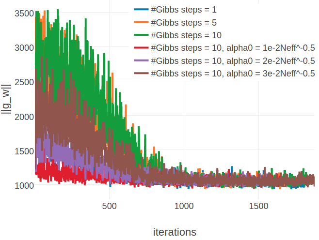
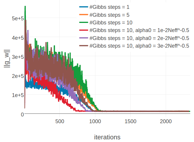
Figure E.15: Monitoring L2 norm of the gradient, $||\nabla_{\w} L\!L(\v^*, \w)||_2$, for protein 1aho_A_00 and 1c75_A_00 during SGD optimization using different number of Gibbs steps and initial learning rates, $\alpha_0$. Number of Gibbs steps is given in the legend, as well as particular choices for the initial learning rate, when not using the default $\alpha_0 = \frac{5e-2}{\sqrt{N_{\text{eff}}}}$. Left Protein 1aho_A_00 has length L=64 and 378 sequences in the alignment (Neff=229) Right Protein 1c75_A_00 has length L=71 and 28078 sequences in the alignment (Neff=16808).

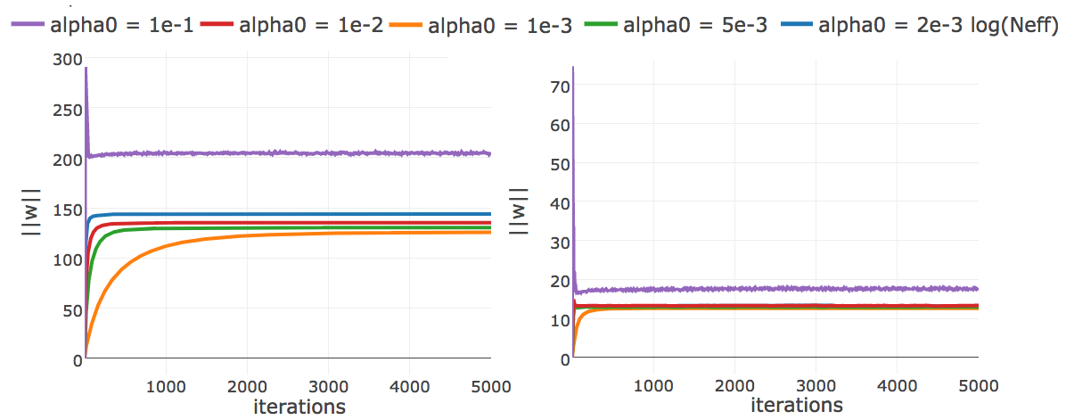
$L2-norm of the coupling parameters, $||\w||_2$, during CD optimization with ADAM with different fixed learning rates (no decay). The learning rate $\alpha_0$ is specified in the legend. Left Protein 1c75A00 has length L=71 and 28078 sequences in the alignment (Neff=16808) Right Protein 1mkcA00 has length L=43 and 142 sequences in the alignment (Neff=96).$

Figure E.16: L2-norm of the coupling parameters, $||\w||_2$, during CD optimization with ADAM with different fixed learning rates (no decay). The learning rate $\alpha_0$ is specified in the legend. Left Protein 1c75A00 has length L=71 and 28078 sequences in the alignment (Neff=16808) Right Protein 1mkcA00 has length L=43 and 142 sequences in the alignment (Neff=96).

$L2-norm of the coupling parameters, $||\w||_2$, during CD optimization with ADAM and different learning rate annealing schedules. The learning rate $\alpha$ is specified with respect to Neff as $\alpha = 2\mathrm{e}{-3}\log(\text{N}_{\text{eff}})$. The learning rate annealing schedule is specified in the legend. Left Convergence plot for protein 1mkc_A_00 having protein length L=43 and 142 sequences in the alignment (Neff=96). Left Protein 1c75A00 has length L=71 and 28078 sequences in the alignment (Neff=16808) Right Protein 1mkcA00 has length L=43 and 142 sequences in the alignment (Neff=96).$ $L2-norm of the coupling parameters, $||\w||_2$, during CD optimization with ADAM and different learning rate annealing schedules. The learning rate $\alpha$ is specified with respect to Neff as $\alpha = 2\mathrm{e}{-3}\log(\text{N}_{\text{eff}})$. The learning rate annealing schedule is specified in the legend. Left Convergence plot for protein 1mkc_A_00 having protein length L=43 and 142 sequences in the alignment (Neff=96). Left Protein 1c75A00 has length L=71 and 28078 sequences in the alignment (Neff=16808) Right Protein 1mkcA00 has length L=43 and 142 sequences in the alignment (Neff=96).$

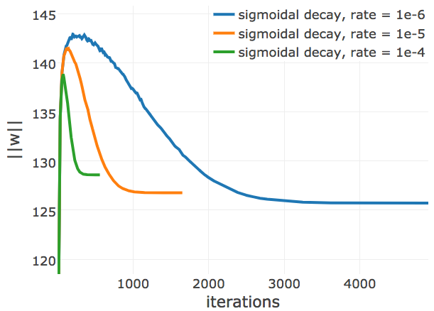
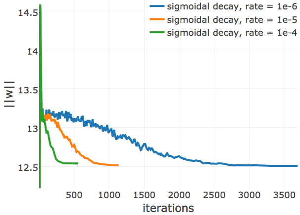
Figure E.17: L2-norm of the coupling parameters, $||\w||_2$, during CD optimization with ADAM and different learning rate annealing schedules. The learning rate $\alpha$ is specified with respect to Neff as $\alpha = 2\mathrm{e}{-3}\log(\text{N}_{\text{eff}})$. The learning rate annealing schedule is specified in the legend. Left Convergence plot for protein 1mkc_A_00 having protein length L=43 and 142 sequences in the alignment (Neff=96). Left Protein 1c75A00 has length L=71 and 28078 sequences in the alignment (Neff=16808) Right Protein 1mkcA00 has length L=43 and 142 sequences in the alignment (Neff=96).

Figure E.18: Precision of top ranked contact predictions for protein 1c75A00. Contact scores are computed as the APC corrected Frobenius norm of the couplings $\wij$. pseudo-likelihood: contact scores computed from pseudo-likelihood. contrastive divergence: contact scores computed from CD optimized with SGD.

Figure E.19: Rolling mean over the mean precision of the L/10 to L top ranked predictions per protein for testset with 2300 proteins. Contact scores computed as APC corrected Frobenius norm over pseudo-likelihood and contrastive divergence couplings. The rolling mean has been computed for the central protein within a window of 20 proteins. Window is shrunk for the proteins at the borders of Neff distribution.

$Contact maps for protein 1ss3A00 and 1c55A00 computed as APC corrected Frobenius norm of the pseudo-likelihood couplings. Contacts are defined according to a $8 \angstrom \Cb$ distance cutoff. Left: predicted contact map and native distance map for protein 1ss3A00 (protein length=50, N=42, Neff=36). Right predicted contact map and native distance map for protein 1c55A00 (protein length = 40, N=115, Neff = 78).$ $Contact maps for protein 1ss3A00 and 1c55A00 computed as APC corrected Frobenius norm of the pseudo-likelihood couplings. Contacts are defined according to a $8 \angstrom \Cb$ distance cutoff. Left: predicted contact map and native distance map for protein 1ss3A00 (protein length=50, N=42, Neff=36). Right predicted contact map and native distance map for protein 1c55A00 (protein length = 40, N=115, Neff = 78).$

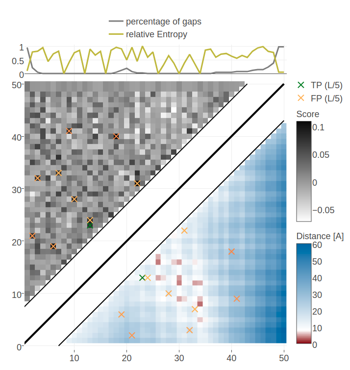
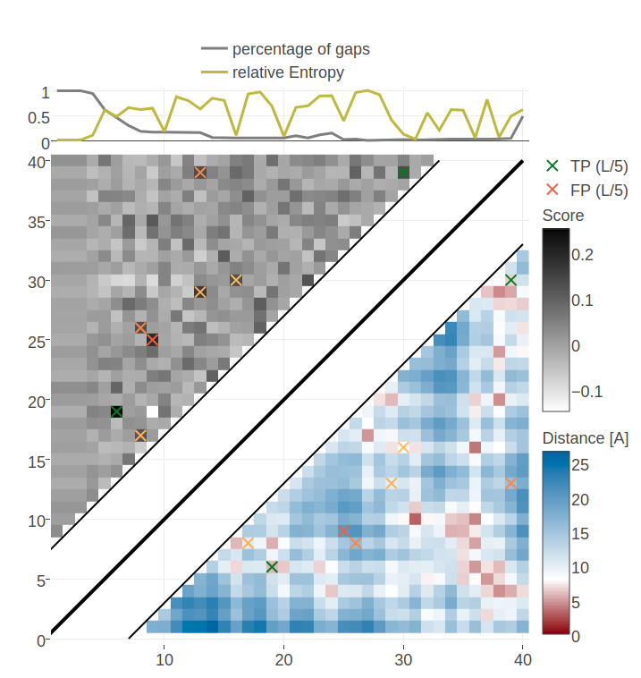
Figure E.20: Contact maps for protein 1ss3A00 and 1c55A00 computed as APC corrected Frobenius norm of the pseudo-likelihood couplings. Contacts are defined according to a $8 \angstrom \Cb$ distance cutoff. Left: predicted contact map and native distance map for protein 1ss3A00 (protein length=50, N=42, Neff=36). Right predicted contact map and native distance map for protein 1c55A00 (protein length = 40, N=115, Neff = 78).

$Contact maps for protein 1c55A00 (protein length = 40, N=115, Neff = 88) computed as APC corrected Frobenius norm of the contrastive-divergence couplings computed with different sample size choices. Contacts are defined according to a $8 \angstrom \Cb$ distance cutoff. Top Left: sample size=0.3neff $\approx$ 23 sequences. Top Right sample size=0.5neff $\approx$ 39 sequences. Bottom Left: sample size=0.8neff $\approx$ 62 sequences. Bottom Right sample size=max(10L,N)=>115 sequences.$ $Contact maps for protein 1c55A00 (protein length = 40, N=115, Neff = 88) computed as APC corrected Frobenius norm of the contrastive-divergence couplings computed with different sample size choices. Contacts are defined according to a $8 \angstrom \Cb$ distance cutoff. Top Left: sample size=0.3neff $\approx$ 23 sequences. Top Right sample size=0.5neff $\approx$ 39 sequences. Bottom Left: sample size=0.8neff $\approx$ 62 sequences. Bottom Right sample size=max(10L,N)=>115 sequences.$ $Contact maps for protein 1c55A00 (protein length = 40, N=115, Neff = 88) computed as APC corrected Frobenius norm of the contrastive-divergence couplings computed with different sample size choices. Contacts are defined according to a $8 \angstrom \Cb$ distance cutoff. Top Left: sample size=0.3neff $\approx$ 23 sequences. Top Right sample size=0.5neff $\approx$ 39 sequences. Bottom Left: sample size=0.8neff $\approx$ 62 sequences. Bottom Right sample size=max(10L,N)=>115 sequences.$ $Contact maps for protein 1c55A00 (protein length = 40, N=115, Neff = 88) computed as APC corrected Frobenius norm of the contrastive-divergence couplings computed with different sample size choices. Contacts are defined according to a $8 \angstrom \Cb$ distance cutoff. Top Left: sample size=0.3neff $\approx$ 23 sequences. Top Right sample size=0.5neff $\approx$ 39 sequences. Bottom Left: sample size=0.8neff $\approx$ 62 sequences. Bottom Right sample size=max(10L,N)=>115 sequences.$

Figure E.21: Contact maps for protein 1c55A00 (protein length = 40, N=115, Neff = 88) computed as APC corrected Frobenius norm of the contrastive-divergence couplings computed with different sample size choices. Contacts are defined according to a $8 \angstrom \Cb$ distance cutoff. Top Left: sample size=0.3neff $\approx$ 23 sequences. Top Right sample size=0.5neff $\approx$ 39 sequences. Bottom Left: sample size=0.8neff $\approx$ 62 sequences. Bottom Right sample size=max(10L,N)=>115 sequences.