3.5 Comparing CD couplings to pLL couplings

A final benchmark over a larger set of proteins (2000 proteins randomly selected from subsets 5 to 10 described in method section 2.6.1) reveals that contact predictions obtained by maximizing the pseudo-likelihood and by optimizing the full likelihood with contrastive divergence perform similar (see Figure 3.22). At any rate it is interesting to not only compare pseudo-likelihood and contrastive divergence based on ovaral performance, but to also have a look at single predictions. In the following, I will examine and compare the predicitons made by both methods for two representative proteins, one with a small alignment and low corresponding Neff value and one with a large alignment and high corresponding Neff value.

Figure 3.22: Mean precision for top ranked contact predictions over 2000 proteins. pseudo-likelihood (APC): contact score is computed as APC corrected Frobenius norm of the couplings computed from pseudo-likelihood. pseudo-likelihood: same as “pseudo-likelihood (APC)” but without APC. contrastive divergence (APC): contact score is computed as APC corrected Frobenius norm of the couplings computed from contrastive-divergence. contrastive divergence: same as “contrastive divergence (APC)” but without APC.

3.5.1 Protein 1c75A00

Protein 1c75A00 has length L=71 and 28078 sequences in the alignment and is among the proteins with the highest number of effective sequences (Neff=16808 > 95th percentile). The contact score (APC corrected Frobenius norm of the couplings \(\wij\)) computed from pseudo-likelihood and contrastive divergence couplings performs equally well (see Appendix Figure E.18). The 14 (=L/5) highest scoring contacts predicted with CD are true positive contacts according to an \(8 \angstrom \Cb\) distance cutoff compared to 13 true positive contacts predicted with pseudo-likelihood. Both methods predict very similar contact maps (see Figure 3.23). The highest scoring predictions (top L/5 contacts marked with croses) are identical except for one contact, which is the false positive contact predicted by the pseudo-likelihood.

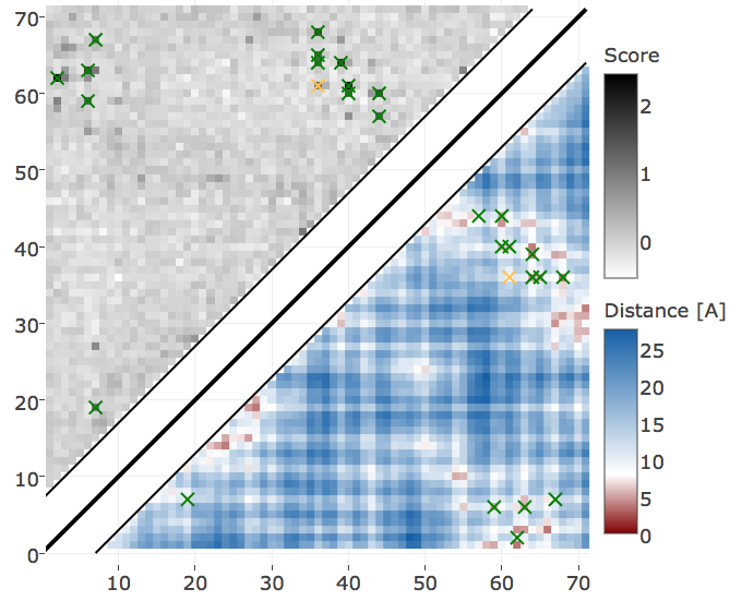
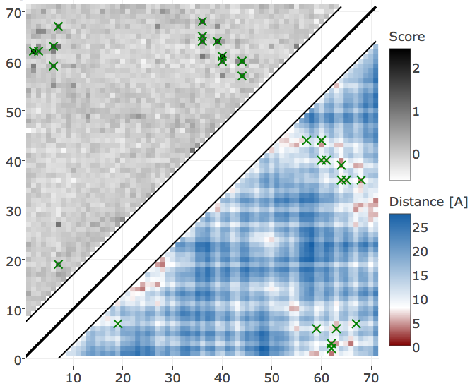
Figure 3.23: Contact maps predicted for protein 1c75A00. Upper left shows predicted contact map and lower right shows the native distance map. Contacts are defined according to a \(8 \angstrom \Cb\) distance cutoff and have been computed as APC corrected Frobenius norm of the couplings. Left Couplings computed from pseudo-likelihood. Right Couplings computed from CD.

The contact maps suggest that both scores are very similar. Indeed, the correlation between both scores is very high (Pearson’s correlation coefficient = 0.98) as can bee seen in the right plot in Figure 3.24. Of course, by applying the average product correction (APC), the scores are normalized with respect to the raw contact scores (=Frobenius norm of couplings \(\wij\)). The left plot in Figure 3.24 shows the contact scores before applying the average product correction. The raw contact scores computed from contrastive divergence couplings are systematically stronger than for pseudo-likelihood. Most likely this effect arises from the weaker regularization that is used with contrastive divergence (\(\lambda_w = 0.1L\)) than compared to pseudo-likelihood optimization (\(\lambda_w = 0.2L\)) (see section 3.3.1).

Figure 3.24: Contact scores computed from pseudo-likelihood and CD couplings for protein 1c75A00. Left Frobenius norm of couplings. Right Frobenius norm + APC of couplings.

However, the contact scores have no meaning by themselfs but merely reflect the confidence of the prediction.
It is more meaningful to compare the ranking of the residue pairs imposed by the scores. The left plot in Figure 3.25 compares the ordered scores of both methods that lie very close to the diagonal which indicates that both distribution are very similar (Kolmogorov-Smirnov pvalue = 0.0078, Spearman rho = 0.947536). A detailed view of the top ranked predictions is given in the right plot in Figure 3.25. The three most confident predictions are identical for both methods. Yet, the ranks of subsequent predictions are swapped by only a few positions which was already evident from the contact maps.

Figure 3.25: Comparing the ranking of highest scoring contacts predicted with pseudo-likelihood and contrastive divergence for protein 1c75A00. Contact scores are computed as APC corrected Frobenius norm of the couplings. Left Q-Q plot. Right Contact scores for the top 71 (=L) predictions from either method. Identical residue pairs are connected with a line. Green indicates identical ranking of the residue pair for both methods. Blue indicates higher ranking of the residue pair for contrastive divergence. Red indicates higher ranking of the residue pair for pseudo-likelihood.

3.5.2 Protein 1ss3A00 and 1c55A00

When analysing sample size it was shown that by randomly selecting 0.3Neff sequences for Gibbs sampling improves performance especially for proteins with small Neff (see Figure 3.12) on a small dataset used for benchmarking (75 proteins per Neff quantile bin). This trend is still visible on the larger test dataset but to a lesser extent (see Figure E.19).

By looking at some of these proteins with small Neff for which the contact score computed from CD couplings performs better than the score computed from pseudo-likelihood couplings, it is striking that CD mainly predicts strongly conserved positions that have high entropy.

For example, for protein 1ss3A00 (protein length=50, Neff=36), CD makes strong predictions for all pairings of the residues (8, 12, 16, 26, 30, 34) (see Figure 3.26). Five of the predicted contacts are actually true contacts. Taking a look at the structure it is revealed that these positions are disulfide bonds which are strongly conserved. Another example is protein 1c55A00 (protein length=40, Neff=78) for which CD makes strong predictions for pairings beetween residues (10, 16, 20, 31, 36, 38). Again, it turns out that the five true positive predictions are disulfide bonds (see bottom plot in Figure 3.26).

Interestingly, pseudo-likelihood does not predict the strongly conserved residues pairs and therefore misses some true contacts (see Appendix Figure E.20). However, when recapitulating the analysis from section 3.3.2 by increasing the sample size step-wise, the contact maps predicted with CD start to resemble those predicted by pseudo-likelihood and the predicted contacts between strongly conserved residues vanish (see Appendix Figure E.21). It was unclear from the analysis of the gradients for different samples sizes in section 3.3.2 why sampling less sequences and consequently a worse gradient estimate results in improved performance for proteins with small Neff. Now it can be hypothesized that the improved performance simply originates from the fact that contacts are predicted between strongly conserved columns.

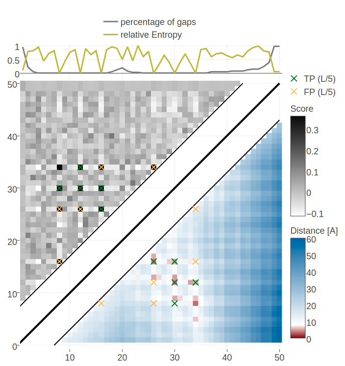
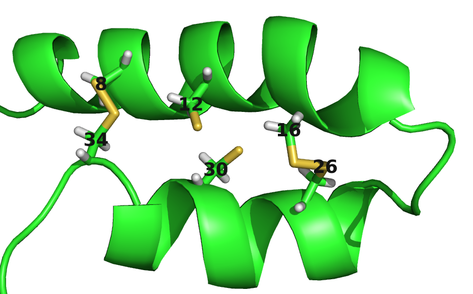
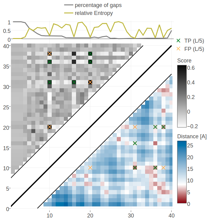
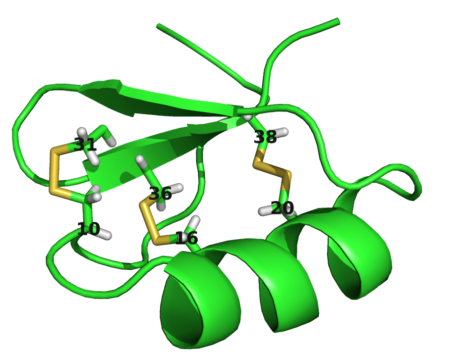
Figure 3.26: Contact maps and structures for protein 1ss3A00 and 1c55A00. Contact scores have been computed as APC corrected Frobenius norm of the CD couplings. Contacts are defined according to a \(8 \angstrom \Cb\) distance cutoff. Upper left: predicted contact map and native distance map for protein 1ss3A00 (protein length=50, N=42, Neff=36). Upper Right: native protein structure of 1ss3A00 with disulfide bonds between residues pairs (8, 34), (12, 30), (16, 26). Lower Left predicted contact map and native distance map for protein 1c55A00 (protein length=40, N=115, Neff=78) Lower Right native protein structure of 1c55A00 with disulfide bonds between residues pairs (10, 31), (16, 36), (20, 38).

This observation stresses the importance to complement coevolutionary analysis in low data scenarios by the use of other sequence derived information, like conservation. The most successfull contact predictors presented in section 1.2.3 integrate features extracted from the MSA because it is known that sequence-based contact prediction is robust when only few sequences are available [86,87].

References

86. Stahl, K., Schneider, M., and Brock, O. (2017). EPSILON-CP: using deep learning to combine information from multiple sources for protein contact prediction. BMC Bioinformatics 18, 303., doi: 10.1186/s12859-017-1713-x.

87. He, B., Mortuza, S.M., Wang, Y., Shen, H.-B., and Zhang, Y. (2017). NeBcon: Protein contact map prediction using neural network training coupled with naïve Bayes classifiers. Bioinformatics., doi: 10.1093/bioinformatics/btx164.