3.3 Tuning the Gibbs Sampling Scheme for Contrastive Divergence

The original CD-k algorithm described by Hinton in 2002 evolves the Markov chains by k=1 Gibbs steps [192]. As described earlier, CD-1 provides a biased estimate of the true gradient because the Markov chains have not reached the stationary distribution [194]. Bengio and Delalleau show that the bias for CD-k kan be understood as a residual term when expressing the log likelihood gradient as an expansion that involves the k-th sample of the Gibbs chain [195,204]. As the number of Gibbs steps, k, goes to infinity the residual term and hence the bias converges to zero and the CD gradient estimate converges to a stochastic estimation of the true likelihood gradient. Indeed, eventhough surprising results have been obtained by evolving the Markov chains for only one Gibbs step, typically CD-k for k>>1 gives more precise results [195]. Furthermore it has been shown, that bias also depends on the mixing rate (rate of convergence) of the chains whereby the mixing rate decreases when model parameters increase [205]. This can lead to divergence of the CD-k solution from optimal solution in a sense that the model systematically gets worse as optimization progresses [206]. Regularization of the parameters offers a solution to this problem, constraining the magnitude of the parameters. A different solution suggested by Bengio and Delalleau is to dynamically increase k when the model parameters increase [195]. These studies analysing the convergence properties and the expected approximation error for CD-k have mainly been conducted for Restricted Boltzmann Machines. It is therefore not clear, whether and to what extent these findings apply to the Potts model.

Several connections of CD to other well known approximation algorithms have been drawn. For example, it can be shown that CD using one Gibbs update step on a randomly selected variable is exactly equivalent to a stochastic maximum pseudo-likelihood estimation [207,208]. Asuncion and colleagues showed further that an arbitrary good approximation to the full likelihood can be reached by applying blocked-Gibbs sampling [209]. CD based on sampling an arbitraty number of variables, has an equivalent stochastic composite likelihood, which is a higher-order generalization of the pseudo-likelihood.

Another variant of CD is PCD, such that the Markov chain is not reinitialized at a data sample every time a new gradient is computed [205]. Instead, the Markov chains are kept persistent that is, they are evolved between successive gradient computations. The fundamental idea behind PCD is that the model changes only slowly between parameter updates given a sufficiently small learning rate. Consequently, the Markov chains will not be pushed too far from equilibrium after each update but rather stay close to the stationary distribution [94,194,205]. Tieleman and others observed that PCD performs better than CD in all practical cases tested, eventhough CD can be faster in the early stages of learning and thus should be preferred when runtime is the limiting factor [94,205,210].

The next sections discuss various modifications of the CD algorithm, such as varying the regularization strength \(\lambda_w\) for constraining the coupling parameters \(\w\), increasing the number of Gibbs sampling steps and varying the number of Markov chains used for sampling. Persistent contrastive divergence is analysed for various combinations of the above mentioned settings and eventually combined with CD-k. Unless noted otherwise, all optimizations will be performed using stochastic gradient descent with the tuned hyperparameters described in the last sections.

3.3.1 Tuning Regularization Coefficients for Contrastive Divergence

For tuning the hyperparameters of the stochastic gradient descent optimizer in the last section 3.2.2, the coupling parameters \(\w\) were constrained by a Gaussian prior \(\mathcal{N}(\w | 0, \lambda_w^{-1} I)\) using the default pseudo-likelihood regularization coefficient \(\lambda_w \eq 1\mathrm{e}{-2}L\) as decscribed in methods section 2.6.5. It is conceivable that CD achieves optimal performance using stronger or weaker regularization than used for pseudo-likelihood optimization. Therefore, I evaluated performance for different regularization coefficients \(\lambda_w \in \{ 5\mathrm{e}{-2}L, 1\mathrm{e}{-1}L, 1\mathrm{e}{-2}L, L\}\) using the previously identified hyperparamters for SGD. The single potentials \(\v\) are not subject to optimization and are kept fixed at their maximum-likelihood estimate \(v^*\) that is derived in eq. (3.16).

As can be seen in Figure 3.10, using strong regularization for the couplings, with \(\lambda_w \eq L\), results in a drastic drop of mean precision. Using weaker regularization, with \(\lambda_w \eq \mathrm{5e}{-2}L\), improves precision for the top \(L/10\) and \(L/5\) predicted contacts but decreases precision when including lower ranked predictions. As a matter of fact, a slightly weaker regularization \(\lambda_w \eq \mathrm{1e}{-1}L\) than the default \(\lambda_w \eq \mathrm{1e}{-2}L\) improves mean precision especially for the top \(L/2\) contacts in such a way, that it is comparable to the pseudo-likelihood performance.

Figure 3.10: Mean precision for top ranked contact predictions over 300 proteins. Contact scores are computed as the APC corrected Frobenius norm of the couplings \(\wij\). pseudo-likelihood: couplings computed with pseudo-likelihood. CD lambda_w = X: couplings computed with CD using L2-regularization on the couplings \(\w\) with regularization coefficient \(\lambda_w\) specified in the legend and keeping the single potentials \(\vi\) fixed at their MLE optimum \(\vi^*\) denoted in eq. (3.16).

As mentioned before, in contrast to pseudo-likelihood optimization the single potentials \(\v\) are not optimized with CD but rather set to their maximum-likelihood estimate as it is obtained in a single position model that is discussed in methods section (3.16). When the single potentials \(\v\) are optimized with CD using the same regularization coefficient \(\lambda_v \eq 10\) as for pseudo-likelihood optimization, performance is almost indistinguishable compared to keeping the single potentials \(\v\) fixed (see Appendix Figure E.12).

3.3.2 Varying the Sample Size

The default Gibbs sampling scheme outlined in method section 3.7.6 involves the random selection of \(10L\) sequences from the input alignment, with \(L\) being protein length, at every iteration of the optimization procedure. These selected sequences are used to initialize the same number of Markov chains. The particular choice of \(10L\) sequences was motivated by the fact that there is a relationship between the precision of contacts predicted from pseudo-likelihood and protein length, at least for alignments with less than \(10^3\) diverse sequences [177]. It has been argued that roughly \(5L\) nonredundant sequences are required to obtain confident predictions that can bet used for protein structure prediction [102].

I analysed whether varying the number of sequences used for the approximation of the gradient via Gibbs sampling affects performance. Randomly selecting only a subset of sequences \(S\) from the \(N\) sequences of the input alignment corresponds to the stochastic gradient descent idea of a minibatch and introduces additional stochasticity over the CD Gibbs sampling process. Using \(S < N\) sequences for Gibbs sampling has the further advantage of decreasing the runtime at each iteration. I evaluated different schemes for the random selection of sequences:

• sampling \(x\)L sequences with \(x \in \{ 1, 5, 10, 50 \}\) without replacement enforcing \(S \eq \min(N, xL)\)
• sampling \(x\)Neff sequences with \(x \in \{ 0.2, 0.3, 0.4 \}\) without replacement

Figure 3.11 illustrates performance for several of the choices. Randomly selecting \(L\) sequences for sampling results in a visible drop in performance. There is no benefit in using more than \(10L\) sequences, especially as sampling more sequences increases runtime per iteration. Specifying the number of sequences for sampling as fractions of Neff generally improves precision slightly over selecting \(10L\) or \(50L\) sequences for sampling. By sampling \(0.3\)Neff sequences, CD does slighty improve over pseudo-likelihood.

Figure 3.11: Mean precision for top ranked contact predictions over 300 proteins. Contact scores are computed as the APC corrected Frobenius norm of the couplings \(\wij\). pseudo-likelihood: couplings computed with pseudo-likelihood. CD sample size = X : contact scores computed from CD with SGD. At every iteration, a particular number of sequences is randomly selected from the input alignmet to initialize the Markoc chains for Gibbs sampling. The number of randomly selected sequences is specified in the legend. It is defined either as multiples of protein length \(L\) or as fraction of the effective number of sequences Neff.

When evaluating performance with respect to the number of effective sequences Neff, it can clearly be noted that the optimal number of randomly selected sequences should be defined as a fraction of Neff. Selecting too many sequences, e.g. \(50L\) for small alignments (left plot in Figure 3.12), or selecting too few sequences, e.g \(1L\) for large alignments (right plot in Figure 3.12), results in a decrease in precision compared to defining the number of sequences as fractions of Neff. Especially small alignments benefit from sample sizes defined as a fraction of Neff with improvements of about three percentage points in precision over pseudo-likelihood.

Figure 3.12: Mean precision for top ranked contact predictions over subsets of 75 proteins, defined according to Neff quartiles. Contact scores are computed as the APC corrected Frobenius norm of the couplings \(\wij\). pseudo-likelihood: contact scores computed from pseudo-likelihood. CD sample size = X : contact scores computed from CD with SGD. The number of randomly selected sequences for the Gibbs sampling process is specified in the legend. It is defined either as multiples of protein length \(L\) or as fraction of the effective number of sequences Neff. Left Subset of 75 proteins with Neff < Q1. Right Subset of 75 proteins with Q3 <= Neff < Q4.

To understand the effect of different choices of sample size it is necessary to look at single proteins. The left plot in Figure 3.13 shows the development of the L2 norm of the gradient for couplings, \(||\nabla_{\w} L\!L(\v^*, \w)||_2\), for protein chain 1c75A00 that is of length 71 and has Neff = 16808. The norm of the gradient decreases during optimization and for increasing choices of the sample size it saturates at decreasing levels. For example, increasing the sample size by a factor 100 (from \(L\) to \(100L\)) leads to an approximately 10-fold reduction of the norm of the gradient at convergence (\(\mathrm{1e}{+5}\) compared to \(\mathrm{1e}{+4}\)), which corresponds to a typical reduction of statistical noise as the square root of the number of samples. It is not feasible to sample the number of sequences at each iteration that would be necessary to reduce the norm of the gradient to near zero!

The previous benchmark showed, that precision of the top ranked contacts does not improve to the same amount as the norm of the gradient decreases when the sample size is increased. Probably, the improved gradient when using a larger sample size helps to finetune the parameters, which only has a negligible effect on the contact score computed as APC corrected Frobenius norm of the couplings \(\wij\). For example, the difference between the parameter norm at convergence for sampling \(10L = 710\) sequences or \(50L = 3550\) sequences is only marginal (see right plot in Figure 3.13), despite a larger difference of the norm of gradients.

It is not clear why an improved gradient estimate due to sampling more sequences results in weaker performance for proteins with small alignments as could be seen in the previous benchmark in Figure 3.12. Protein 1ahoA00, that has length 64 and an alignment of 378 sequences (Neff=229), achieves a mean precision of 0.44 over the top \(0.1L\) - \(L\) contacts when using all \(N \eq 378\) sequences for sampling. When only \(0.3N_{\textrm{eff}} \eq 69\) sequences are used in the sampling procedure, 1ahoA00 achieves a mean precision of 0.62. Appendix Figure E.13 shows the course of the norm of the gradient and the norm of coupling parameters during optimization for this protein. Similarly as it has been observed for protein 1c75A00, the norm of the gradient converges towards smaller values when more sequences are used in the Gibbs sampling process and the improved gradient is supposed to lead to a better approximation of the likelihood. One explanation for this obvious discrepancy could be some effect of overfitting. Eventhough a regularizer is used for optimization and the norm of coupling parameters actually is smaller when using a larger sample size (see the right plot in Appendix Figure E.13).

Figure 3.13: Monitoring parameter norm and gradient norm for protein 1c75A00 during SGD using different sample sizes. Protein 1c75A00 has length L=71 and 28078 sequences in the alignment (Neff=16808). The number of sequences, that is used for Gibbs sampling to approximate the gradient, is given in the legend with 1L = 71 sequences, 5L = 355 sequences, 10L = 710 sequences, 50L = 3550 sequences, 100L = 7100 sequences, 0.2Neff = 3362 sequences, 0.3Neff = 5042 sequences, 0.4Neff = 6723 sequences. Left L2-norm of the gradients for coupling parameters, \(||\nabla_{\w} L\!L(\v^*, \w)||_2\) (without contribution of regularizer). Right L2-norm of the coupling parameters \(||\w||_2\).

3.3.3 Varying the number of Gibbs Steps

As discussed earlier, it has been pointed out in the literature that using \(k>1\) Gibbs steps for sampling sequences gives more precise results at the cost of longer runtimes per gradient evaluation [195,205]. I analysed the impact on performance when the number of Gibbs steps is increased to 5 and 10. As can be seen in Figure 3.14, increasing the number of Gibbs steps does result in a slight drop of performance. When evaluating precision with respect to Neff it can be found that using more Gibbs sampling steps is especially disadvantageous for large alignments (see Appendix Figure E.14).

Figure 3.14: Mean precision for top ranked contact predictions over 300 proteins. Contact scores are computed as the APC corrected Frobenius norm of the couplings \(\wij\). pseudo-likelihood: contact scores computed from pseudo-likelihood. CD #Gibbs steps = X: contact scores computed from CD optimized with SGD and evolving each Markov chain using the number of Gibbs steps specified in the legend.

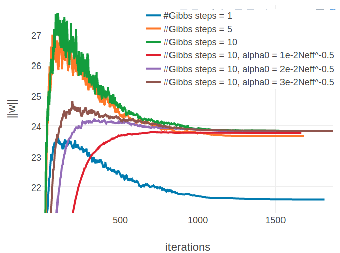
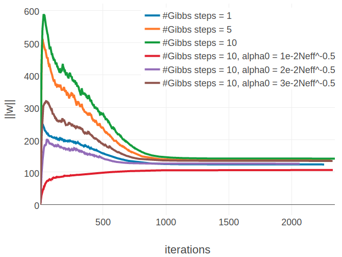
When evaluating single proteins, it can be observed that for proteins with small alignments the L2 norm of the parameters, \(||\w||_2\), converges towards a different offset when using more than one Gibbs steps (see left plot in Figure 3.15). Naturally, the Markov chains can wander further away from their initialization when they are evolved over a longer time which results in a stronger gradient at the beginning of the optimization. Therefore and because the initial learning rate has been optimized for sampling with one Gibbs step, the parameter norm overshoots the optimum at the beginning. Even when lowering the initial learning rate from \(\alpha_0 = \frac{5e-2}{\sqrt{N_{\text{eff}}}}\) to \(\alpha_0 \in \left \{ \frac{3e-2}{\sqrt{N_{\text{eff}}}}, \frac{2e-2}{\sqrt{N_{\text{eff}}}} , \frac{1e-2}{\sqrt{N_{\text{eff}}}} \right \}\), the SGD optimizer evidently approaches a different optimum. Surprisingly, the different optimum that is found for proteins with small alignments has no substantial impact on precision, as becomes evident from Figure E.14. For proteins with large alignments it can be observed that there is not one alternative solution to the parameters, but depending on the number of Gibbs steps and on the initial learning rate, \(\alpha_0\), the L2 norm over parameters converges towards various different offsets (see right plot in Figure 3.15). It is not clear how these observations can be interpreted, in particular given the fact, that the L2 norm of gradients, \(||\nabla_{\w} L\!L(\v^*, \w)||_2\), converges to the identical offset for all settings regardless of alignment size (see Appendix Figure E.15). Optimizing CD with 10 Gibbs steps and using a smaller initial learning rate, \(\alpha0 = \frac{2e-2}{\sqrt{N_{\text{eff}}}}\), does not have an overal impact on mean precision as can be seen in Figure 3.14.

Figure 3.15: Monitoring parameter norm, \(||\w||_2\), for protein 1aho_A_00 and 1c75_A_00 during SGD optimization using different number of Gibbs steps and initial learning rates, \(\alpha_0\). Number of Gibbs steps is given in the legend, as well as particular choices for the initial learning rate, when not using the default \(\alpha_0 = \frac{5e-2}{\sqrt{N_{\text{eff}}}}\). Left Protein 1aho_A_00 has length L=64 and 378 sequences in the alignment (Neff=229) Right Protein 1c75_A_00 has length L=71 and 28078 sequences in the alignment (Neff=16808).

3.3.4 Persistent Contrastive Divergence

Finally I analysed, whether evolving the Markov chains over successive iterations, which is known as PCD, does improve performance [205]. Several empirical studies have shown that PCD performs superior compared to CD-1 and also to CD-10 [205,210]. In the literatur is has been pointed out that PCD needs to use small learning rates because in order to sample from a distribution close to the stationary distribution, the parameters cannot change too rapidly. However, using smaller learning rates not only increases runtime but also requires tuning of the learning rate and learning rate schedule once again. Since it has been found, that CD is faster in learning at the beginning of the optimization, I tested a compromise, that uses CD-1 at the beginning of the optimization and when learning slows down, PCD is switched on. Concretely, PCD is switched on, when the relative change of the norm of coupling parameters, \(||\w||_2\), falls below \(\epsilon \in \{\mathrm{1e}{-3}, \mathrm{1e}{-5}\}\) while the convergence criterion is not altered and convergence is assumed when the relative change falls below \(\epsilon \eq \mathrm{1e}{-8}\). As a result, the model will already have approached the optimum when PCD is switched on so that the coupling parameters \(\w\) will mot change to quickly over many updates.

Figure 3.16: Mean precision for top ranked contact predictions over 300 proteins. Contact scores are computed as the APC corrected Frobenius norm of the couplings \(\wij\). pseudo-likelihood: contact scores computed from pseudo-likelihood. pCD: contact scores computed from PCD optimized with SGD using the hyperparameters that have been found to work optimal with CD as described throughout the last sections. pCD #Gibbs steps = 10: same as pCD, but evolving the Gibbs chain for 10 steps. pCD start = 1e-3: SGD optimization starts by optimizing the full likelihood using the CD gradient estimate and switches to the PCD gradient estimate once the relative change of L2 norm of parameters has fallen below \(\epsilon \eq \mathrm{1e}{-3}\) evaluated over the last 10 iterations. pCD start = 1e-5: same as ‘pCD start = 1e-3’, but with \(\epsilon \eq \mathrm{1e}{-5}\).

Figure 3.16 shows the mean precision of top ranked contacts on the validation set computed with several PCD variants that perform almost equally well. Evolving the Gibbs chains for k=10 steps results in a slight drop in performance, just as it has been observed for CD. Optimizing the full likelihoood with CD and switiching to PCD at a later stage of optimization does also not have a notable impact on performance.

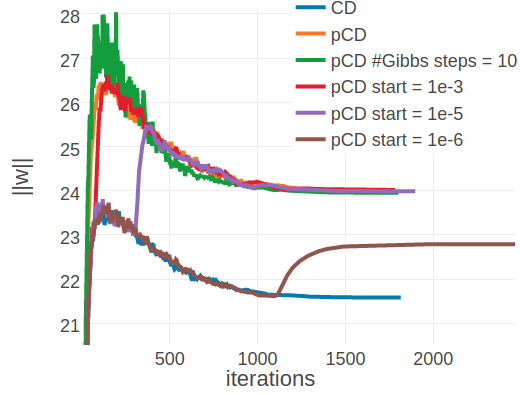
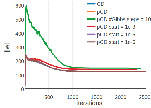
Again it is insightful to observe the optimization progresss for single proteins. For protein 1ahoA00, with low Neff=229, the PCD model converges to the same coupling norm offset (\(||\w||_2 \approx 24\)) as the CD model using 5 and 10 Gibbs steps (see left plot in Figure 3.17 compared to left plot in 3.15). It can also be seen that when PCD is switched on at a later stage of optimization the coupling norm jumps from the CD-1 level to the PCD level. The different optimum that is found for proteins with small alignments does not seem to affect predictive performance. Interestingly, convergence behaves differently for protein 1c75A00, that has high Neff=16808 (see right plot in Figure 3.17). PCD using one Gibbs step converges to a different coupling norm offset than CD-1 and PCD using ten Gibbs steps. However, when PCD is switched on later during optimization the model either ends up in the CD-1 (switch at \(\epsilon \eq 1e-5\) or \(\epsilon \eq 1e-6\)) or in the PCD optimum (switch at \(\epsilon \eq 1e-3\)). The cause for this behaviour is unclear, yet it has no noticable impact on overal performance.

Figure 3.17: Monitoring parameter norm, \(||\w||_2\), for protein 1ahoA00 and 1c75A00 during SGD optimization of different objectives. Left Protein 1ahoA00 has length L=64 and 378 sequences in the alignment (Neff=229) Right Protein 1c75A00 has length L=71 and 28078 sequences in the alignment (Neff=16808). CD contrastive divergence using 1 Gibbs step. pCD persistent contrastive divergence using 1 Gibbs step. pCD #Gibbs steps = 10 persistent contrastive divergence using 10 Gibbs steps. pCD start = 1e-3, pCD start = 1e-5: same as in Figure 3.16 pCD start = 1e-6: same as ‘pCD start = 1e-3’, but with \(\epsilon \eq \mathrm{1e}{-6}\).

Against expectations from the findings in literature, neither CD-k with k>1 Gibbs steps nor PCD does improve performance with respect to precision of the top ranked contact predictions. Swersky and colleagues ellaborated on various choices of hyperparameters (e.g momentum, averaging, regularization, etc.) for training Restricted Boltzmann Machines as classifiers with CD-k and PCD [210]. They found many subtleties that need to be explored and can play a crucial role for successfull training. In section 3.2.2 I manually tuned the learning rate and annealing schedule for stoachstic gradient descent to be used with CD-1. It is plausible, that these settings are not optimal for CD-k with k>1 Gibbs steps and PCD and require tuning once again. Because hyperparameter optimization with stochastic gradient descent is a time-consuming task, in the following, I applied the popular ADAM stochastic gradient descent optimizer that does in theory not require tuning many hyperparameters [211].

References

192. Hinton, G.E. (2002). Training Products of Experts by Minimizing Contrastive Divergence. Neural Comput. 14, 1771–1800., doi: doi:10.1162/ 089976602760128018.

194. Fischer, A., and Igel, C. (2012). An Introduction to Restricted Boltzmann Machines. Lect. Notes Comput. Sci. Prog. Pattern Recognition, Image Anal. Comput. Vision, Appl. 7441, 14–36., doi: 10.1007/978-3-642-33275-3_2.

195. Bengio, Y., and Delalleau, O. (2009). Justifying and Generalizing Contrastive Divergence. Neural Comput. 21, 1601–21., doi: 10.1162/neco.2008.11-07-647.

204. Ma, X., and Wang, X. (2016). Average Contrastive Divergence for Training Restricted Boltzmann Machines. Entropy 18, 35., doi: 10.3390/e18010035.

205. Tieleman, T. (2008). Training Restricted Boltzmann Machines using Approximations to the Likelihood Gradient. Proc. 25th Int. Conf. Mach. Learn. 307, 7., doi: 10.1145/1390156.1390290.

206. Fischer, A., and Igel, C. (2010). Empirical Analysis of the Divergence of Gibbs Sampling Based Learning Algorithms for Restricted Boltzmann Machines. In Artif. neural networks – icann 2010 (Springer, Berlin, Heidelberg), pp. 208–217., doi: 10.1007/978-3-642-15825-4_26.

207. Hyvärinen, A. (2006). Consistency of pseudolikelihood estimation of fully visible Boltzmann machines.

208. Hyvarinen, A. (2007). Connections Between Score Matching, Contrastive Divergence, and Pseudolikelihood for Continuous-Valued Variables. IEEE Trans. Neural Networks 18, 1529–1531., doi: 10.1109/TNN.2007.895819.

209. Asuncion, A.U., Liu, Q., Ihler, A.T., and Smyth, P. (2010). Learning with Blocks: Composite Likelihood and Contrastive Divergence. Proc. Mach. Learn. Res. 9, 33–40.

94. Murphy, K.P. (2012). Machine Learning: A Probabilistic Perspective (MIT Press).

210. Swersky, K., Chen, B., Marlin, B., and Freitas, N. de (2010). A tutorial on stochastic approximation algorithms for training Restricted Boltzmann Machines and Deep Belief Nets. In 2010 inf. theory appl. work. (IEEE), pp. 1–10., doi: 10.1109/ITA.2010.5454138.

177. Anishchenko, I., Ovchinnikov, S., Kamisetty, H., and Baker, D. (2017). Origins of coevolution between residues distant in protein 3D structures. Proc. Natl. Acad. Sci., 201702664., doi: 10.1073/pnas.1702664114.

102. Kamisetty, H., Ovchinnikov, S., and Baker, D. (2013). Assessing the utility of coevolution-based residue-residue contact predictions in a sequence- and structure-rich era. Proc. Natl. Acad. Sci. U. S. A. 110, 15674–9., doi: 10.1073/pnas.1314045110.

211. Kingma, D., and Ba, J. (2014). Adam: A Method for Stochastic Optimization.