3.2 Optimizing the Full Likelihood

Given the likelihood gradient estimates obtained with CD, the full negative log likelihood can now be minimized using a gradient descent optimization algorithm. Gradient descent algorithms are used to find the minimum of an objective function with respect to its parametrization by iteratively updating the parameters values in the opposite direction of the gradient of the objective function with respect to these parameters. Stochastic gradient descent (SGD) is a variant thereof that uses a stochastic estimate of the gradient whose average over many updates approaches the true gradient. The stochasticity is commonly obtained by evaluating a random subsample of the data at each iteration. For CD stochasticity additionally arises from the Gibbs sampling process in order to obtain a gradient estimate in the first place.

As a consequence of stochasticity, the gradient estimates are noisy, resulting in parameter updates with high variance and strong fluctuations of the objective function. These fluctuations enable stochastic gradient descent to escape local minima but also complicate finding the exact minimum of the objective function. By slowly decreasing the step size of the parameter updates at every iteration, stochastic gradient descent most likely will converge to the global minimum for convex objective functions [196–198]. However, choosing an optimal step size for parameter updates as well as finding the optimal annealing schedule offers a challenge and needs manual tuning [199,200]. If the step size is chosen too small, progress will be unnecessarily slow, if it is chosen too large, the optimum will be overshot and can cause the system to diverge (see Figure 3.2). Further complications arise from the fact that different parameters often require different optimal step sizes, because the magnitude of gradients might vary considerably for different parameters, e.g. because of sparse data.

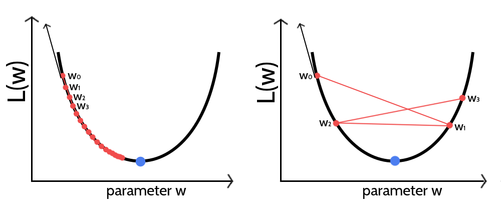
Figure 3.2: Visualization of gradient descent optimization of an objective function \(L(w)\) for different step sizes \(\alpha\). The blue dot marks the minimum of the objective function. The direction of the gradient at the initial parameter estimate \(w_0\) is given as black arrow. The updated parameter estimate \(w_1\) is obtained by taking a step of size \(\alpha\) into the opposite direction of the gradient. Left If the step size is too small the algorithm will require too many iterations to converge. Right If the step size is too large, gradient descent will overshoot the minimum and can cause the system to diverge.

Unfortunately, it is neither possible to use second order optimization algorithms nor sophisticated first order algorithms like conjugate gradients to optimize the full likelihood of the Potts model. While the former class of algorithms requires (approximate) computation of the second partial derivatives, the latter requires evaluating the objective function in order to identify the optimal step size via linesearch, both being computationally too demanding.

The next subsections describe the hyperparameter tuning for stochastic gradient descent, covering the choice of the convergence criterion and finding the optimal learning rate annealing schedule.

3.2.1 Convergence Criterion for Stochastic Gradient Descent

In theory the gradient descent algorithm has converged and the optimum of the objective function has been reached when the gradient becomes zero. In practice the gradients will never be exactly zero, especially due to the stochasticity of the gradient estimates when using stochastic gradient descent with CD. For this reason, it is crucial to define a suitable convergence criterion that can be tested during optimization and once the criterion is met, convergence is assumed and the algorithm is stopped. Typically, the objective function (or a related loss function) is periodically evaluated on a validation set and the optimizer is halted whenever the function value saturates or starts to increase. This technique is called early stopping and additionally prevents overfitting [201,202]. Unfortunately, we cannot compute the full likelihood function due to its complexity and need to define a different convergence criterion.

One possibility is to stop learning when the L2 norm of the gradient for the coupling parameters \(||\nabla_{\w} L\!L(\v^*, \w)||_2\) is close to zero [203]. However, when using a finite number of sequences for sampling, the norm of the gradient does not converge to zero but towards a certain offset as it is described in section 3.3.2. Convergence could also be monitored as the relative change of the norm of gradients within a certain number of iterations. Optimization will be stopped when the relative change becomes negligibly small, that is when the gradient norm has reached a plateau. As gradient estimates are very noisy with stochastic gradient descent, gradient fluctuations complicate the proper assessment of this criterion.

Instead of the gradient, it is also possible to observe the relative change of the norm of parameter estimates \(||\w||_2\) over several iterations and stop learning when it falls below a small threshold \(\epsilon\), \[\begin{equation} \frac{||\w_{t-x}||_2 - ||\w_t||_2}{||\w_{t-x}||_2} < \epsilon \; . \tag{3.3} \end{equation}\]

This measure is less noisy than subsequent gradient estimates because the magnitude of parameter updates is bounded by the learning rate.

For stochastic gradient descent the optimum is a moving target and the gradient will start oscillating when approaching the optimum. Therefore, another idea is to monitor the direction of the partial derivatives. However, this theoretical assumption is complicated by the fact that gradient oscillations are also typically observed when the parameter surface contains narrow valleys or generally when the learning rate is too big, as it is visualized in the right plot in Figure 3.2. When optimizing high-dimensional problems using the same learning rate for all dimensions, it is likely that parameters converge at different speeds [196] leading to oscillations that could either originate from convergence or yet too large learning rates. As can be seen in Figure 3.3, the percentage of parameters for which the derivate changes direction within the last \(x\) iterations is usually high and varies for different proteins. Therefore it is not a good indicator of convergence. When using the adaptive learning rate optimizer ADAM, the momentum term is an interfering factor for assessing the direction of partial derivatives. Parameters will be updated into the direction of a smoothed historical gradient and oscillations, regardless of which origin, will be dampened. It is therefore hard to define a general convergence criteria based on the direction of derivatives that can distinguish these different scenarios.

Figure 3.3: Percentage of parameters for which the derivate has changed its direction (i.e. the sign) during the previous \(x\) iterations (\(x\) is specified in the legend). Optimization is performed with SGD using the optimal hyperparameters defined in section 3.2.2 and using a regularization coefficient \(\lambda_w \eq 0.1L\) (see section 3.3.1) and using one step of Gibbs sampling. Optimization is stopped when the relative change over the L2-norm of parameter estimates \(||\w||_2\) over the last \(x\) iterations falls below the threshold of \(\epsilon \eq 1e-8\). Development has been monitored for two different proteins, Left 1c75A00 (protein length = 71, number sequences = 28078, Neff = 16808) Right 1ahoA00 (protein length = 64, number sequences = 378, Neff = 229).

Of course, the simplest strategy to assume convergence is to specify a maximum number of iterations for the optimization procedure, which also ensures that the algorithm will stop eventually if none of the other convergence criteria is met.

3.2.2 Tuning Hyperparameters of Stochastic Gradient Descent Optimizer

The coupling parameters \(\w\) will be updated at each time step \(t\) by taking a step of size \(\alpha\) along the direction of the negative gradient of the regularized full log likelihood, \(- \nabla_w \LLreg(\v^*,\w)\), that has been approximated with CD,

\[\begin{equation} \w_{t+1} = \w_t - \alpha \cdot \nabla_w \LLreg(\v^*,\w) \; . \end{equation}\]

In order to get a first intuition of the optimization problem, I tested initial learning rates \(\alpha_0 \in \{1\mathrm{e}{-4}, 5\mathrm{e}{-4}, 1\mathrm{e}{-3}, 5\mathrm{e}{-3}\}\) with a standard learning rate annealing schedule, \(\alpha = \frac{\alpha_0}{1 + \gamma \cdot t}\) where \(t\) is the time step and \(\gamma\) is the decay rate that is set to 0.01[197].

Figure 3.4 shows the mean precision for top ranked contacts computed from pseudo-likelihood couplings and from CD couplings optimized with stochastic gradient descent using the four different learning rates. Overall, mean precision for CD contacts is lower than for pseudo-likelihood contacts, especially when using the smallest (\(\alpha_0 \eq 1\mathrm{e}{-4}\)) and largest (\(\alpha_0 \eq 5\mathrm{e-}{3}\)) learning rate.

Figure 3.4: Mean precision for top ranked contact predictions over 300 proteins. Contact scores are computed as the APC corrected Frobenius norm of the couplings \(\wij\). pseudo-likelihood: couplings computed with pseudo-likelihood. CD alpha0 = X: couplings computed with CD using stochastic gradient descent with different initial learning rates \(\alpha_0\) (see legend).

By looking at individual proteins it becomes evident that the optimal learning rate depends on alignment size. Figure 3.5 displays the development of the L2 norm of the coupling parameters, \(||\w||_2\), during optimization using different learning rates for two proteins with different alignment sizes. The left plot shows protein 1c75A00 that has a large alignment with 28078 sequences (Neff = 16808) while the right plot shows protein 1ahoA00 that has a small alignment with 378 sequences (Neff = 229). For protein 1ahoA00 and using a small initial learning rate \(\alpha_0 \eq \mathrm{1e-4}\), the optimization runs very slowly and does not converge within tha maximum number of 5000 iterations. Using a large initial learning rate \(\alpha_0 \eq \mathrm{5e-3}\) results in slighly overshooting the optimum at the beginning of the optimization but with the learning rate decaying over time the parameter estimates converge. In contrast, for protein 1c75A00, the choice of learning rate has a more pronounced effect. With a small initial learning rate \(\alpha_0 \eq \mathrm{1e-4}\) the optimization runs slowly but almost converges within 5000 iterations. A large initial learning rate \(\alpha_0 \eq \mathrm{5e-3}\) lets the parameters diverge quickly and the optimum cannot be recovered. With learning rates \(\alpha_0 \eq \mathrm{5e-4}\) and \(\alpha_0 \eq \mathrm{1e-3}\), the optimum is well overshot at the beginning of the optimization but the parameter estimates eventually converge as the learning rate decreases over time.

These observations can be explained by the fact that the magnitude of the gradient scales with the number of sequences in the alignment. The gradient is computed from amino acid counts as explained before. Therefore, alignments with many sequences will generally produce larger gradients than alignments with few sequences, especially at the beginning of the optimization procedure when the difference in amino acid counts between sampled and observed sequences is largest. Following these observations, I defined the initial learning rate \(\alpha_0\) as a function of Neff,

\[\begin{equation} \alpha_0 = \frac{5\mathrm{e}{-2}}{\sqrt{N_{\text{eff}}}} \; . \tag{3.4} \end{equation}\]

For small Neff, e.g. 5th percentile of the distribution in the dataset \(\approx 50\), this definition of the learning rate yields \(\alpha_0 \approx 7\mathrm{e}{-3}\) and for large Neff, e.g. 95th percentile \(\approx 15000\), this yields \(\alpha_0 \approx 4\mathrm{e}{-4}\). These values for \(\alpha_0\) lie in the optimal range that has been observed for the two representative proteins in Figure 3.4. With the initial learning rate defined as a function of Neff, precision slightly improves over the previous fixed learning rates (see Appendix Figure E.1). All following analyses are conducted using the Neff-dependent initial learning rate.

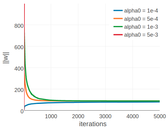
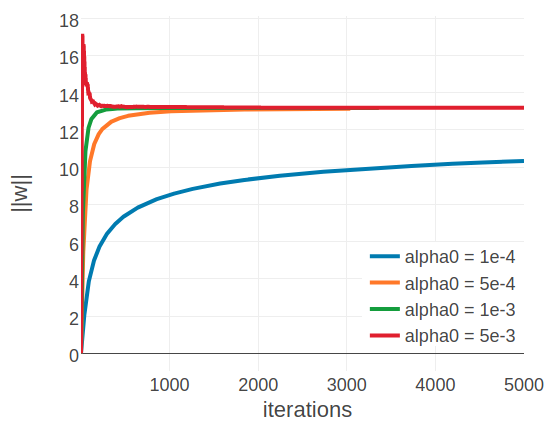
Figure 3.5: Convergence plots for two proteins during SGD optimization with different learning rates and convergence measured as L2-norm of the coupling parameters \(||\w||_2\). Linear learning rate annealing schedule has been used with decay rate \(\gamma=0.01\) and initial learning rates \(\alpha_0\) have been set as specified in the legend. Left 1c75A00 (protein length = 71, number sequences = 28078, Neff = 16808). Figure is cut at the yaxis at \(||\w||_2=1000\), but learning rate of \(5\mathrm{e}{-3}\) reaches \(||\w||_2 \approx 9000\). Right 1ahoA00 (protein length = 64, number sequences = 378, Neff = 229)

In a next step, I evaluated the following learning rate annealing schedules and decay rates using the Neff-dependent initial learning rate given in eq. (3.4):

• default linear learning rate schedule \(\alpha = \frac{\alpha_0}{1 + \gamma t}\) with \(\gamma \in \{1\mathrm{e}{-3}, 1\mathrm{e}{-2}, 1\mathrm{e}{-1}, 1 \}\)
• square root learning rate schedule \(\alpha = \frac{\alpha_0}{\sqrt{1 + \gamma t}}\) with \(\gamma \in \{1\mathrm{e}{-2}, 1\mathrm{e}{-1}, 1 \}\)
• sigmoidal learning rate schedule \(\alpha_{t+1} = \frac{\alpha_{t}}{1 + \gamma t}\) with \(\gamma \in \{1\mathrm{e}{-6}, 1\mathrm{e}{-5}, 1\mathrm{e}{-4}, 1\mathrm{e}{-3}\}\)
• exponential learning rate schedule \(\alpha_{t+1} = \alpha_0 \cdot\exp(- \gamma t)\) with \(\gamma \in \{5\mathrm{e}{-4}, 1\mathrm{e}{-4}, 5\mathrm{e}{-3}\}\)

The learning rate annealing schedules are visualized for different decay rates in Appendix Figure E.2. Optimizing CD with SGD using any of the learning rate schedules listed above yields on average lower precision for the top ranked contacts than the pseudo-likelihood contact score. Several learning rate schedules perform almost equally and yield a mean precision that is about one to two percentage below the mean precision for the pseudo-likelihood contact score (see Figure 3.6): a linear learning rate schedule with decay rate \(\gamma \eq 1\mathrm{e}{-2}\), a sigmoidal learning rate schedule with decay rates \(\gamma \eq 1\mathrm{e}{-5}\) or \(\gamma \eq 1\mathrm{e}{-6}\) and an exponential learning rate schedule with decay rates \(\gamma \eq 1\mathrm{e}{-3}\) or \(\gamma \eq 1\mathrm{e}{-5}\). The square root learning rate schedule gives ovarall bad results and does not lead to convergence because the learning rate decays slowly at later time steps. The benchmark plots for all learning rate schedules are shown in Appendix Figures E.3, E.4, E.5, E.6.

Figure 3.6: Mean precision for top ranked contact predictions over 300 proteins. Contact scores are computed as the APC corrected Frobenius norm of the couplings \(\wij\). pseudo-likelihood: couplings computed with pseudo-likelihood. CD: couplings computed with CD using stochastic gradient descent with an initial learning rate defined with respect to Neff. Learning rate annealing schedules and decay rates are specified in the legend.

In contrast to the findings regarding the initial learning rate earlier, an optimal decay rate can be defined independent of the alignment size. Figure 3.7 shows the development of the L2 norm of the coupling parameters, \(||\w||_2\), during optimization for the same two representative proteins with small and large alignments as before. Convergence for protein 1ahoA00, having small Neff=229, is robust against the particular choice of learning rate schedule and decay rate and the presumed optimum at \(||w||_2 \approx 13.2\) is reached regardless of the learning rate annealing schedule (see right plot in Figure 3.7). For protein 1c75A00, with high Neff=16808, the choice of the learning rate schedule has a notable impact on the rate of convergence. Using a linear schedule, the learning rate decays quickly but then converges to a certain offset, which effectively prevents further optimization progress and the presumed optimum at \(||w||_2 \approx 90\) is not reached within 5000 iterations. Learning rate schedules that decay slower but decay continously for 5000 iterations, such as an exponential schedule with \(\gamma \eq 1\mathrm{e}{-3}\) or a sigmoidal schedule with \(\gamma \eq 1\mathrm{e}{-6}\), guide the parameter estimates close to the expected optimum. Therefore, learning rate schedules with an exponential or sigmoidal decay can be used with proteins having low Neffs as well as high Neffs.

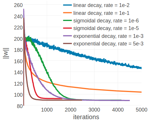
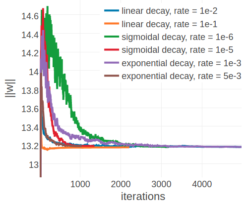
Figure 3.7: L2-norm of the coupling parameters \(||\w||_2\) during stochastic gradient descent optimization with different learning rates schedules. The initial learning rate \(\alpha_0\) is defined with respect to Neff as given in eq. (3.4). Learning rate schedules and decay rates are used according to the legend. Left 1c75A00 (protein length = 71, number sequences = 28078, Neff = 16808). Right 1ahoA00 (protein length = 64, number sequences = 378, Neff = 229)

Another aspect worth considering is runtime and it can be observed that the different learning rate annealing schedules differ in convergence speed. Figure 3.8 shows the distribution over the number of iterations until convergence for SGD optimizations with five different learning rate schedules that yield similar performance. The optimization converges on average within less than 2000 iterations only when using either a sigmoidal learning rate annealing schedule with decay rate \(\gamma \eq 1\mathrm{e}{-5}\) or an exponential learning rate annealing schedule with decay rate \(\gamma \eq 5\mathrm{e}{-3}\), On the contrary, the distribution of iterations until convergence has a median of 5000 when using a linear learning rate annealing schedule with \(\gamma \eq 1\mathrm{e}{-2}\) or an exponential schedule with decay rate \(\gamma \eq 1\mathrm{e}{-3}\). Under these considerations, I chose a sigmoidal learning rate schedule with \(\gamma \eq 5\mathrm{e}{-6}\) for all further analysis.

Figure 3.8: Distribution of the number of iterations until convergence for SGD optimizations of CD for different learning rate schedules. Convergence is reached when the relative difference of parameter norms, \(||\w||_2\), over the last five iterations falls below \(\epsilon \eq 1e-8\). Initial learning rate \(\alpha_0\) is defined with respect to Neff as given in eq. (3.4) and maximum number of iterations is set to 5000. Learning rate schedules and decay rates are specified in the legend.

Finally, I checked whether altering the convergence criteria has notable impact on performance. Per default, optimization is stopped whenever the relative change of the L2 norm over coupling parameters, \(||\w||_2\), over the last 5 iterations falls below a small value \(\epsilon < 1e-8\) as denoted in eq. (3.3). Figure 3.9 shows that the mean precision over proteins is robust to different settings of the number of iterations over which the relative change is computed. The convergence rate is mildly affected by the different settings. Optimization converges on average within 1697, 1782 and 1917 iterations, when computing the relative change of the parameter norm over the previous 2,5 and 10 iterations, respectively (see Appendix Figure E.11). For all following analysis, I chose 10 to be the number of iterations over which the convergence criterion is computed.

Figure 3.9: Mean precision for top ranked contact predictions over 300 proteins. Contact scores are computed as the APC corrected Frobenius norm of the couplings \(\wij\). pseudo-likelihood: couplings computed with pseudo-likelihood. #previous iterations = X: couplings computed with CD using stochastic gradient descent with an initial learning rate defined with respect to Neff and the sigmoidal learning rate schedule with \(\gamma \eq 5\mathrm{e}{-6}\). The relative change of the L2 norm over coupling parameters, \(||\w||_2\), is evaluated over the previous X iterations (specified in the legend) and convergence is assumed when the relative change falls below a small value \(\epsilon \eq 1e-8\).

References

196. Ruder, S. (2017). An overview of gradient descent optimization algorithms. arXiv.

198. Bottou, L. (2010). Large-Scale Machine Learning with Stochastic Gradient Descent. 177–186., doi: 10.1007/978-3-7908-2604-3_16.

199. Schaul, T., Zhang, S., and Lecun, Y. (2013). No More Pesky Learning Rates. arXiv.

200. Zeiler, M.D. (2012). ADADELTA: An Adaptive Learning Rate Method. 6.

201. Bengio, Y. (2012). Practical Recommendations for Gradient-Based Training of Deep Architectures. In Neural networks: Tricks of the trade (Springer Berlin Heidelberg), pp. 437–478., doi: 10.1007/978-3-642-35289-8_26.

202. Mahsereci, M., Balles, L., Lassner, C., and Hennig, P. (2017). Early Stopping without a Validation Set. arXiv.

203. Carreira-Perpiñán, M. a, and Hinton, G.E. (2005). On Contrastive Divergence Learning. Artif. Intell. Stat. 0, 17., doi: 10.3389/conf.neuro.10.2009.14.121.

197. Bottou, L. (2012). Stochastic Gradient Descent Tricks. In Neural networks: Tricks of the trade (Springer, Berlin, Heidelberg), pp. 421–436., doi: 10.1007/978-3-642-35289-8_25.