PhD thesis: residue-residue contact prediction

5.3 Training the Hyperparameters in the Likelihood Function of Contact States

Solving the integral in eq. (5.2) as described in in detail in method section 5.7.3, yields the likelihood function of contact states, $p(\X | \c)$. It contains the hyperparameters of the prior over couplings, $p(\wij|\cij)$, which is modelled as a mixture of $K$ 400-dimensional Gaussians with component weights that depend on the contact state.

The hyperparameters are trained by minimizing the negative logarithm of the likelihood over a set of training MSAs as described in detail in method section 5.7.11. The MAP estimates of the coupling parameters $\wij^*$ are needed to compute the Hessian of the regularized Potts model likelihood, which again is needed for the Gaussian approximation to the regularized likelihood (see method section 5.7.2). For that purpose, I trained the hyperparameters by utilizing couplings $\wij^*$ obtained from pseudo-likelihood maximization as well as couplings $\wij^*$ obtained by maximizing the full likelihood with contrastive divergence (CD).

In the following I present the results of learning the hyperparameters for the coupling prior modelled as a Gaussian mixture with $K \in \{3,5,10\}$ Gaussian components with diagonal precision matrices $\Lk$ and a zero-component that is fixed at $\mu_0=0$ on datasets of different sizes (see method section 5.7.11.1 for details).

5.3.1 Training Hyperparameters for a Gaussian Mixture with Three Components

Training of the hyperparameters for three component Gaussian mixtures based on pseudo-likelihood and contrastive divergence couplings converged after several hundreds of iterations. The inferred hyperparameters obtained by several independent optimization runs and on the datasets of different size (10000, 100000, 3000000, 500000 residue pairs per contact class) are consistent. The following analysis is conducted for the training on the dataset with 300,000 residue pairs per contact class and by using pseudo-likelihood couplings for estimation of the Hessian.

Figure 5.1 shows the statistics of the inferred hyperparameters. The zeroth component, with $\mu_0=0$ has a weight of 0.88 for the non-contact class, whereas it has only weight 0.51 for the contact class. This is expected given that the couplings $\wijab$ for non-contacts have a much tighter distribution around zero than contacts. Component 2 has on average the highest standard deviations and for several dimensions this component is located far off from zero, e.g. dimension EE has $\mu_2(\text{EE}) \eq -0.57$ or ER has $\mu_2(\text{ER}) \eq 0.43$. Therefore, it is not surprising that component 2 has a low weight for non-contacts ($g_2(0) \eq 0.0026$) but a higher weight for contacts ($g_2(1) \eq 0.13$). Statistics of the Gaussian mixture hyperparameters learned on the other datasets is shown in Appendix Figures G.2 and G.3. The inferred hyperparameters for the Gaussian mixture model based on couplings optimized with contrastive divergence are consistent with the estimates obtained by using pseudo-likelihood couplings as can be seen in Appendix Figures G.5 ans G.4.

$Statistics for the hyperparameters, $\gamma_k(\cij)$, $\muk$ and $\Lk$ of a three component Gaussian mixture obtained after 331 iterations. Trained on 300,000 residue pairs per contact class and using pseudo-likelihood couplings to estimate the Hessian. Left Component weights $\gamma_k(\cij)$ for residue pairs not in physical contact ($\cij \eq 0$) and true contacts ($\cij \eq 1$). Center Distribution of the 400 elements in the mean vectors $\muk$. Right Distribution of the 400 standard deviations corresponding to the square root of the diagonal of $\Lk^{-1}$.$

Figure 5.1: Statistics for the hyperparameters, $\gamma_k(\cij)$, $\muk$ and $\Lk$ of a three component Gaussian mixture obtained after 331 iterations. Trained on 300,000 residue pairs per contact class and using pseudo-likelihood couplings to estimate the Hessian. Left Component weights $\gamma_k(\cij)$ for residue pairs not in physical contact ($\cij \eq 0$) and true contacts ($\cij \eq 1$). Center Distribution of the 400 elements in the mean vectors $\muk$. Right Distribution of the 400 standard deviations corresponding to the square root of the diagonal of $\Lk^{-1}$.

Figure 5.2 shows several one-dimensional projections of the 400 dimensionl Gaussian mixture with three components. Generally, the Gaussian mixture learned for residue pairs that are not in contact is much narrower and almost symmetrically centered around zero. The Gaussian mixture for contacts, by contrast is much broader and often skewed. For the aliphatic amino acid pair (V,I), the Gaussian mixture for both contacts and non-contacts is very symmetrical and much narrower compared for example to the Gaussian mixtures for the aromatic amino acid pair (F,W), which also has symmetrical distributions. In contrast, the distribution of couplings for amino acid pairs (E,R) and (E,E) has strong tails for positive and negative values respectively. The one-dimensional projections of the Gaussian mixture model greatly resemble the empirical distributions of couplings illustrated in Figure 2.3 and in Figure 2.6 in chapter 2. The Gaussian mixtures learned on larger datasets produce very similar distributions (see Appendix Figures G.6 and G.7). Likewise, the distributions from the Gaussian mixture models that have been learned based on contrastive divergence couplings are also very similar and shown in Appendix Figure G.8.

$Visualisation of one-dimensional projections of the three-component Gaussian mixture model for the contact-dependent coupling prior. Hyperparameters, $\gamma_k(\cij)$, $\muk$ and $\Lk$, have been trained on 300,000 residue pairs per contact class and using pseudo-likelihood couplings to estimate the Hessian. Green solid line: Gaussian mixture for contacts. Blue solid line: Gaussian mixture for non-contacts. Black solid line: regularization prior with $\lambda_1 \eq 0.2L$ with L being protein length and assumed $L\eq150$. Dashed lines: unweighted probability densities of Gaussian components with color code specified in the legend. Top Left One dimensional projection for pair (V,I). Top Right One dimensional projection for pair (F,W). Bottom Left One dimensional projection for pair (E,R). Bottom Right One dimensional projection for pair (E,E).$

Figure 5.2: Visualisation of one-dimensional projections of the three-component Gaussian mixture model for the contact-dependent coupling prior. Hyperparameters, $\gamma_k(\cij)$, $\muk$ and $\Lk$, have been trained on 300,000 residue pairs per contact class and using pseudo-likelihood couplings to estimate the Hessian. Green solid line: Gaussian mixture for contacts. Blue solid line: Gaussian mixture for non-contacts. Black solid line: regularization prior with $\lambda_1 \eq 0.2L$ with L being protein length and assumed $L\eq150$. Dashed lines: unweighted probability densities of Gaussian components with color code specified in the legend. Top Left One dimensional projection for pair (V,I). Top Right One dimensional projection for pair (F,W). Bottom Left One dimensional projection for pair (E,R). Bottom Right One dimensional projection for pair (E,E).

Distributions from the two-dimensional projection of the Gaussian mixture model are shown in Figure 5.3 for several pairs of couplings. The type of paired couplings has been chosen to allow a direct comparison to the empirical distributions in Figure 2.13 in chapter 2. The top left plot shows the distribution of sampled coupling values according to the Gaussian mixture model for contacts for amino acid pairs (E,R) and (R,E). Component 2 has a weight of 0.13 for contacts and is mainly responsible for the positive coupling between (E,R) and (R,E). The amino acid pairs (E,E) and (R,E) are negatively coupled and again component 2 generates the strongest couplings far off zero as can be seen in the top right plot. The plots at the bottom of Figure 5.3 show the distribution of sampled couplings for amino acid pairs (I,L) and (V,I) according to the Gaussian mixture model for contacts (component weight $g_k(1)$) as well as for non-contacts (component weight $g_k(0)$). The coupling distribution for contacts is symmetrically centered around zero just as the distribution for non-contacts. Because of the higher weight of component 2, the distribution for contacts is much broader than the distribution for non-contacts. The two-dimensional distributions of sampled couplings obtained from the set of Gaussian mixture hyperparameters that have been learned based on contrastive divergence couplings, are very similar and shown in Appendix Figure G.9

$Visualisation of two-dimensional projections of the three-component Gaussian mixture model for the contact-dependent coupling prior.Hyperparameters, $\gamma_k(\cij)$, $\muk$ and $\Lk$, have been trained on 300,000 residue pairs per contact class and using pseudo-likelihood couplings to estimate the Hessian. 10,000 paired couplings have been sampled from the Gaussian mixture model. The different colors represent the generating component and color code is specified in the legend. Top Left Two-dimensional projection for pairs (E,R) and (R-E) for contacts (using component weight $g_k(1)$). Top Right Two- dimensional projection for pairs (E,E) and (R,E) for contacts (using component weight $g_k(1)$). Bottom Left Two-dimensional projection for pairs (I,L) and (V,I) for contacts (using component weight $g_k(1)$). Bottom Right Two-dimensional projection for pair (I,L) and (V,I) for non-contacts (using component weight $g_k(0)$).$

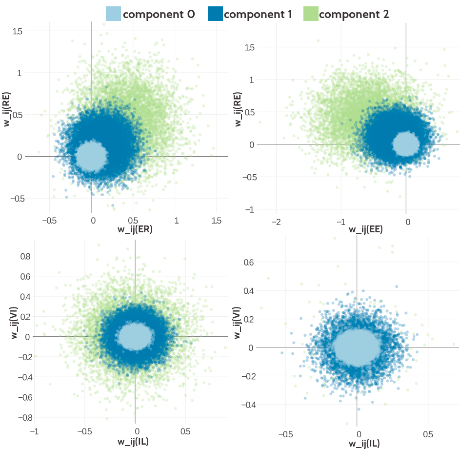
Figure 5.3: Visualisation of two-dimensional projections of the three-component Gaussian mixture model for the contact-dependent coupling prior.Hyperparameters, $\gamma_k(\cij)$, $\muk$ and $\Lk$, have been trained on 300,000 residue pairs per contact class and using pseudo-likelihood couplings to estimate the Hessian. 10,000 paired couplings have been sampled from the Gaussian mixture model. The different colors represent the generating component and color code is specified in the legend. Top Left Two-dimensional projection for pairs (E,R) and (R-E) for contacts (using component weight $g_k(1)$). Top Right Two- dimensional projection for pairs (E,E) and (R,E) for contacts (using component weight $g_k(1)$). Bottom Left Two-dimensional projection for pairs (I,L) and (V,I) for contacts (using component weight $g_k(1)$). Bottom Right Two-dimensional projection for pair (I,L) and (V,I) for non-contacts (using component weight $g_k(0)$).

5.3.2 Training Hyperparameters for a Gaussian Mixture with Five and Ten Components

The increased complexity of training five or even ten instead of three component Gaussian mixtures does not only result in longer runtimes until convergence but also slows down runtime per iteration. The optimization runs for five and ten component Gaussian mixtures did not converge within 2000 iterations. Nevertheless, the obtained hyperparameters and resulting Gaussian mixture are consistent, as will be shown in the following.

Figure 5.4 and 5.5 show the statistics of the inferred hyperparameters for a five and ten component Gaussian mixture, respectively. Similary to three component Gaussian mixtures, the zeroth component receives a high weight for couplings from residue pairs that are not in physical contact ($g_0(0) \eq 0.93$ for five component mixture and $g_0(0) \eq 0.87$ for ten component mixture). There is a second component with a noteworthy contribution to the Gaussian mixture for non-contact couplings (component 3 with $g_3(0) \eq 0.07$ for five component mixture and component 9 with $g_9(0) \eq 0.13$ for ten component mixture). These two components are also the strongest components for the Gaussian mixture representing couplings from contacting residue pairs. The inferred hyperparameters for Gaussian mixture models based on couplings optimized with contrastive divergence are consistent with the estimates obtained by using pseudo-likelihood couplings as can be seen in Appendix Figures G.10 and G.11.

$Statistics for the hyperparameters, $\gamma_k(\cij)$, $\muk$ and $\Lk$ of a five component Gaussian mixture obtained after 1134 iterations. Trained on 300,000 residue pairs per contact class and using pseudo-likelihood couplings to estimate the Hessian. Left Component weights $\gamma_k(\cij)$ for residue pairs not in physical contact ($\cij \eq 0$) and true contacts ($\cij \eq 1$). Center Distribution of the 400 elements in the mean vectors $\muk$. Right Distribution of the 400 standard deviations corresponding to the square root of the diagonal of $\Lk^{-1}$.$

Figure 5.4: Statistics for the hyperparameters, $\gamma_k(\cij)$, $\muk$ and $\Lk$ of a five component Gaussian mixture obtained after 1134 iterations. Trained on 300,000 residue pairs per contact class and using pseudo-likelihood couplings to estimate the Hessian. Left Component weights $\gamma_k(\cij)$ for residue pairs not in physical contact ($\cij \eq 0$) and true contacts ($\cij \eq 1$). Center Distribution of the 400 elements in the mean vectors $\muk$. Right Distribution of the 400 standard deviations corresponding to the square root of the diagonal of $\Lk^{-1}$.

$SStatistics for the hyperparameters, $\gamma_k(\cij)$, $\muk$ and $\Lk$ of a ten component Gaussian mixture obtained after 700 iterations. Trained on 300,000 residue pairs per contact class and using pseudo-likelihood couplings to estimate the Hessian. X-axis represents the ten components numbered from 0 to 9. Top Component weights $\gamma_k(\cij)$ for residue pairs not in physical contact ($\cij \eq 0$) and true contacts ($\cij \eq 1$). Middle Distribution of the 400 elements in the mean vectors $\muk$. Bottom Distribution of the 400 standard deviations corresponding to the square root of the diagonal of $\Lk^{-1}$.$ $SStatistics for the hyperparameters, $\gamma_k(\cij)$, $\muk$ and $\Lk$ of a ten component Gaussian mixture obtained after 700 iterations. Trained on 300,000 residue pairs per contact class and using pseudo-likelihood couplings to estimate the Hessian. X-axis represents the ten components numbered from 0 to 9. Top Component weights $\gamma_k(\cij)$ for residue pairs not in physical contact ($\cij \eq 0$) and true contacts ($\cij \eq 1$). Middle Distribution of the 400 elements in the mean vectors $\muk$. Bottom Distribution of the 400 standard deviations corresponding to the square root of the diagonal of $\Lk^{-1}$.$ $SStatistics for the hyperparameters, $\gamma_k(\cij)$, $\muk$ and $\Lk$ of a ten component Gaussian mixture obtained after 700 iterations. Trained on 300,000 residue pairs per contact class and using pseudo-likelihood couplings to estimate the Hessian. X-axis represents the ten components numbered from 0 to 9. Top Component weights $\gamma_k(\cij)$ for residue pairs not in physical contact ($\cij \eq 0$) and true contacts ($\cij \eq 1$). Middle Distribution of the 400 elements in the mean vectors $\muk$. Bottom Distribution of the 400 standard deviations corresponding to the square root of the diagonal of $\Lk^{-1}$.$

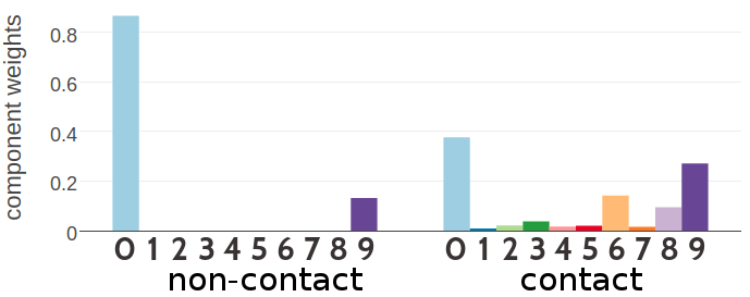
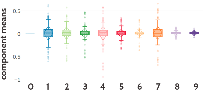
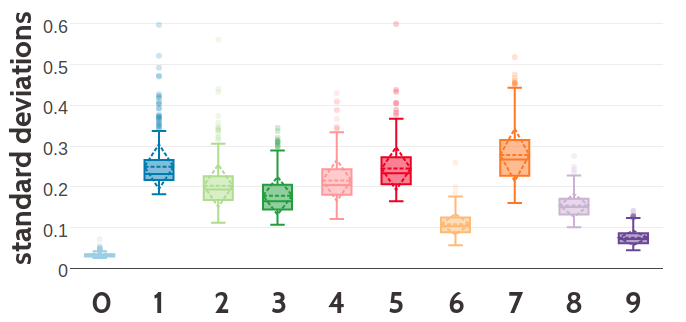
Figure 5.5: SStatistics for the hyperparameters, $\gamma_k(\cij)$, $\muk$ and $\Lk$ of a ten component Gaussian mixture obtained after 700 iterations. Trained on 300,000 residue pairs per contact class and using pseudo-likelihood couplings to estimate the Hessian. X-axis represents the ten components numbered from 0 to 9. Top Component weights $\gamma_k(\cij)$ for residue pairs not in physical contact ($\cij \eq 0$) and true contacts ($\cij \eq 1$). Middle Distribution of the 400 elements in the mean vectors $\muk$. Bottom Distribution of the 400 standard deviations corresponding to the square root of the diagonal of $\Lk^{-1}$.

Figure 5.6 compares the one-dimensional projections of the 400 dimensionl Gaussian mixtures with five and ten components for the amino acid pairs (V,I) and (E,R). The general observations regarding the shape of the Gaussian mixture for couplings from contacts and non-contacts that have been found for the three component mixture also apply here. Generally, the Gaussian mixture for couplings from non-contacts is narrower in the five and ten component mixtures than in the three component Gaussian mixture model. Thereby, the differentiation between contacts and non-contacts is enhanced because the ratio between the Gaussian mixture probability distribution for contacts and non-contacts increases. Furthermore, whereas in the three component model only two components would contribute to defining the tails of the distribution for couplings from contacts, now there are more components that can refine the tails. For example, in the case of amino acid pair (E,R) all but the zeroth component, which is fixed at zero, are shifted towards positive values. In the case of amino acid pair (V,I) the components are shifted towards both positive and negative values. Overall, the Gaussian mixtures with five and ten components seem to refine the modelling of the coupling distributions compared to the simpler three component model. The same observations apply to the one-dimensional projections of the Gaussian mixtures inferred based on contrastive divergence couplings only that the resultant mixtures are even narrower (see Appendix Figure G.12).

$Visualisation of one-dimensional projections of the five and ten component Gaussian mixture model for the contact-dependent coupling prior. Hyperparameters, $\gamma_k(\cij)$, $\muk$ and $\Lk$, have been trained on 300,000 residue pairs per contact class and using pseudo-likelihood couplings to estimate the Hessian. Green solid line: Gaussian mixture for contacts. Blue solid line: Gaussian mixture for non-contacts. Black solid line: regularization prior with $\lambda_1 \eq 0.2L$ with L being protein length and assumed $L\eq150$. Dashed lines represent the unweighted Gaussian mixture components. Top Left One dimensional projection for pair (V,I) from the five component model. Top Right One dimensional projection for pair (V,I) from the ten component model. Bottom Left One dimensional projection for pair (E,R) from the five component model. Bottom Right One dimensional projection for pair (E,R) from the ten component model.$

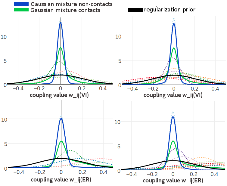
Figure 5.6: Visualisation of one-dimensional projections of the five and ten component Gaussian mixture model for the contact-dependent coupling prior. Hyperparameters, $\gamma_k(\cij)$, $\muk$ and $\Lk$, have been trained on 300,000 residue pairs per contact class and using pseudo-likelihood couplings to estimate the Hessian. Green solid line: Gaussian mixture for contacts. Blue solid line: Gaussian mixture for non-contacts. Black solid line: regularization prior with $\lambda_1 \eq 0.2L$ with L being protein length and assumed $L\eq150$. Dashed lines represent the unweighted Gaussian mixture components. Top Left One dimensional projection for pair (V,I) from the five component model. Top Right One dimensional projection for pair (V,I) from the ten component model. Bottom Left One dimensional projection for pair (E,R) from the five component model. Bottom Right One dimensional projection for pair (E,R) from the ten component model.

Two-dimensional projections of the Gaussian mixture with five and ten components are shown in Figure 5.7 for different pairs of couplings. The distributions resemble the ones learned for the Gaussian mixture with three components. However, it is visible that the zeroth component is narrower for the five and ten component Gaussian mixture and that the additional components model particular parts of the distribution. For example, component 9 in the ten component Gaussian mixture model produces couplings for amino acid pairs (E-R) and (R-E) that are close to zero in both dimensions or even slightly negative. The Gaussian mixture of the coupling prior that has been learned based on couplings computed with contrastive divergence in general produces distributions that are narrower which is expected given the hyperparameter statistics and the observations from the univariate distributions.

$Visualisation of two-dimensional projections of the five and ten component Gaussian mixture model for the contact-dependent coupling prior. Hyperparameters, $\gamma_k(\cij)$, $\muk$ and $\Lk$, have been trained on 300,000 residue pairs per contact class and using pseudo-likelihood couplings to estimate the Hessian. 10,000 paired couplings have been sampled from the Gaussian mixture model. The color of a sampled coupling pair represents the Gaussian mixture component that has generated this sample point. Color code is specified in the legend. Top Left Two-dimensional projection for pairs (E,R) and (R-E) for contacts (using component weight $g_k(1)$) from the five component Gaussian mixture model. Top Right Two-dimensional projection for pairs (E,R) and (R-E) for contacts (using component weight $g_k(1)$) from the ten component Gaussian mixture model. Bottom Left Two-dimensional projection for pair (I,L) and (V,I) for non-contacts (using component weight $g_k(0)$) from the five component Gaussian mixture model. Bottom Right Two-dimensional projection for pair (I,L) and (V,I) for non-contacts (using component weight $g_k(0)$) from the ten component Gaussian mixture model.$

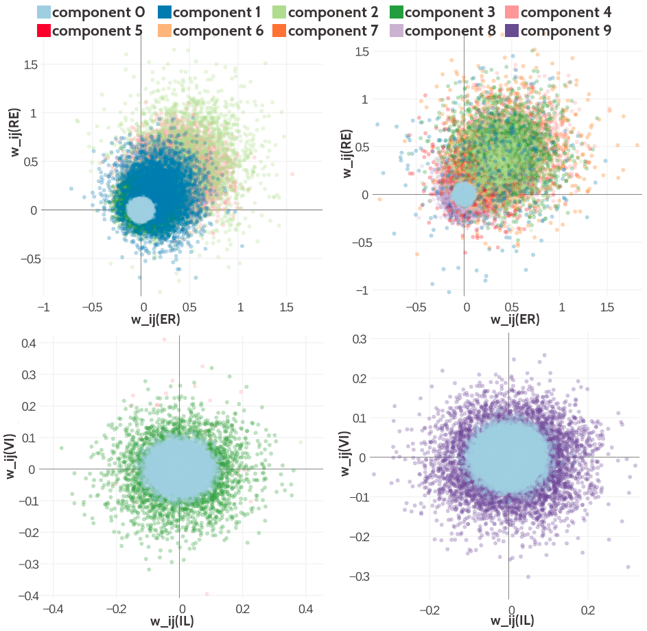
Figure 5.7: Visualisation of two-dimensional projections of the five and ten component Gaussian mixture model for the contact-dependent coupling prior. Hyperparameters, $\gamma_k(\cij)$, $\muk$ and $\Lk$, have been trained on 300,000 residue pairs per contact class and using pseudo-likelihood couplings to estimate the Hessian. 10,000 paired couplings have been sampled from the Gaussian mixture model. The color of a sampled coupling pair represents the Gaussian mixture component that has generated this sample point. Color code is specified in the legend. Top Left Two-dimensional projection for pairs (E,R) and (R-E) for contacts (using component weight $g_k(1)$) from the five component Gaussian mixture model. Top Right Two-dimensional projection for pairs (E,R) and (R-E) for contacts (using component weight $g_k(1)$) from the ten component Gaussian mixture model. Bottom Left Two-dimensional projection for pair (I,L) and (V,I) for non-contacts (using component weight $g_k(0)$) from the five component Gaussian mixture model. Bottom Right Two-dimensional projection for pair (I,L) and (V,I) for non-contacts (using component weight $g_k(0)$) from the ten component Gaussian mixture model.

In conclusion it can be found that training of the hyperparameters for the Gaussian mixtures of the contact-dependent couplig prior seems to be robust. Training consistently yields comparable hyperparameter settings and the Gaussian mixtures produce similar distributions regardless of the dataset size and repeated independent runs. The Gaussian mixture repeatedly reproduce the empirical distribution of couplings shown in Figure 2.13 in chapter 2 very well. Of course it must be noted that the empirical distributions do not take the uncertainty of the inferred couplings into account. They are computed for high evidence couplings as explained in method section 2.6.7 and therefore do not provide a completely correct reference. Besides, looking at two dimensional projections of the 400 dimensional Gaussian mixture model can only provide a limited view of the high-dimensional interdependencies. Another restricting issue is runtime. The more components define the Gaussian mixture, the longer it takes to train the model per iteration and the more iterations it takes to reach convergence. However, without reaching convergence it cannot be assured that the identified hyperparameters for five and ten component Gaussian mixtures represent optimal estimates.