G Bayesian statistical model for contact prediction

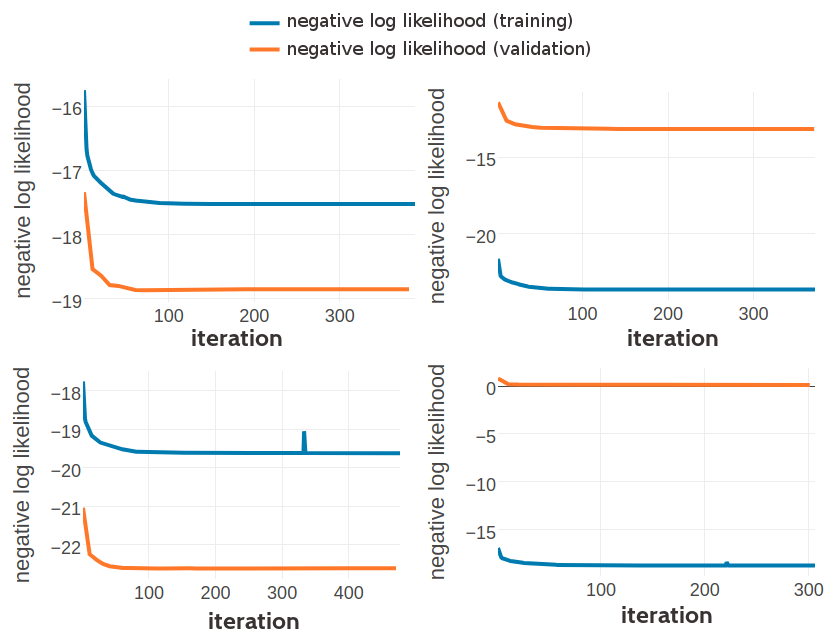
Monitoring the negative log likelihood during optimization of three component Gaussian mixture using pseudo-likelihood couplings to estimate the Hessian. Top Left: Training set contains 10,000 residue pairs per contact class. Converged after 388 iterations. Top Right: Training set contains 100,000 residue pairs per contact class. Converged after 371 iterations. Bottom Left: Training set contains 300,000 residue pairs per contact class. Bottom Right: Training set contains 500,000 residue pairs per contact class.

Figure G.1: Monitoring the negative log likelihood during optimization of three component Gaussian mixture using pseudo-likelihood couplings to estimate the Hessian. Top Left: Training set contains 10,000 residue pairs per contact class. Converged after 388 iterations. Top Right: Training set contains 100,000 residue pairs per contact class. Converged after 371 iterations. Bottom Left: Training set contains 300,000 residue pairs per contact class. Bottom Right: Training set contains 500,000 residue pairs per contact class.

$Statistics for the hyperparameters, $\gamma_k(\cij)$, $\muk$ and $\Lk$ obtained after 388 iterations. Trained on 10,000 residue pairs per contact class for a three component Gaussian mixture and using pseudo-likelihood couplings to estimate the Hessian. Left Component weights $\gamma_k(\cij)$ for residue pairs not in physical contact ($\cij \eq 0$) and true contacts ($\cij \eq 1$). Center Distribution of the 400 elements in the mean vectors $\muk$. Right Distribution of the 400 standard deviations corresponding to the square root of the diagonal of $\Lk^{-1}$.$

Figure G.2: Statistics for the hyperparameters, $\gamma_k(\cij)$, $\muk$ and $\Lk$ obtained after 388 iterations. Trained on 10,000 residue pairs per contact class for a three component Gaussian mixture and using pseudo-likelihood couplings to estimate the Hessian. Left Component weights $\gamma_k(\cij)$ for residue pairs not in physical contact ($\cij \eq 0$) and true contacts ($\cij \eq 1$). Center Distribution of the 400 elements in the mean vectors $\muk$. Right Distribution of the 400 standard deviations corresponding to the square root of the diagonal of $\Lk^{-1}$.

$Statistics for the hyperparameters, $\gamma_k(\cij)$, $\muk$ and $\Lk$ obtained after 371 iterations. Trained on 100,000 residue pairs per contact class for a three component Gaussian mixture and using pseudo-likelihood couplings to estimate the Hessian. Left Component weights $\gamma_k(\cij)$ for residue pairs not in physical contact ($\cij \eq 0$) and true contacts ($\cij \eq 1$). Center Distribution of the 400 elements in the mean vectors $\muk$. Right Distribution of the 400 standard deviations corresponding to the square root of the diagonal of $\Lk^{-1}$.$

Figure G.3: Statistics for the hyperparameters, $\gamma_k(\cij)$, $\muk$ and $\Lk$ obtained after 371 iterations. Trained on 100,000 residue pairs per contact class for a three component Gaussian mixture and using pseudo-likelihood couplings to estimate the Hessian. Left Component weights $\gamma_k(\cij)$ for residue pairs not in physical contact ($\cij \eq 0$) and true contacts ($\cij \eq 1$). Center Distribution of the 400 elements in the mean vectors $\muk$. Right Distribution of the 400 standard deviations corresponding to the square root of the diagonal of $\Lk^{-1}$.

$Statistics for the hyperparameters, $\gamma_k(\cij)$, $\muk$ and $\Lk$ obtained after optimization of the likelihood function of contact states for 336 iterations. Trained on 10,000 residue pairs per contact class for a three component Gaussian mixture and using contrastive divergence couplings to estimate the Hessian. Left Component weights $\gamma_k(\cij)$ for residue pairs not in physical contact ($\cij \eq 0$) and true contacts ($\cij \eq 1$). Center Distribution of the 400 elements in the mean vectors $\muk$. Right Distribution of the 400 standard deviations corresponding to the square root of the diagonal of $\Lk^{-1}$.$

Figure G.4: Statistics for the hyperparameters, $\gamma_k(\cij)$, $\muk$ and $\Lk$ obtained after optimization of the likelihood function of contact states for 336 iterations. Trained on 10,000 residue pairs per contact class for a three component Gaussian mixture and using contrastive divergence couplings to estimate the Hessian. Left Component weights $\gamma_k(\cij)$ for residue pairs not in physical contact ($\cij \eq 0$) and true contacts ($\cij \eq 1$). Center Distribution of the 400 elements in the mean vectors $\muk$. Right Distribution of the 400 standard deviations corresponding to the square root of the diagonal of $\Lk^{-1}$.

$Statistics for the hyperparameters, $\gamma_k(\cij)$, $\muk$ and $\Lk$ obtained after optimization of the likelihood function of contact states for 377 iterations. Trained on 100,000 residue pairs per contact class for a three component Gaussian mixture and using contrastive divergence couplings to estimate the Hessian. Left Component weights $\gamma_k(\cij)$ for residue pairs not in physical contact ($\cij \eq 0$) and true contacts ($\cij \eq 1$). Center Distribution of the 400 elements in the mean vectors $\muk$. Right Distribution of the 400 standard deviations corresponding to the square root of the diagonal of $\Lk^{-1}$.$

Figure G.5: Statistics for the hyperparameters, $\gamma_k(\cij)$, $\muk$ and $\Lk$ obtained after optimization of the likelihood function of contact states for 377 iterations. Trained on 100,000 residue pairs per contact class for a three component Gaussian mixture and using contrastive divergence couplings to estimate the Hessian. Left Component weights $\gamma_k(\cij)$ for residue pairs not in physical contact ($\cij \eq 0$) and true contacts ($\cij \eq 1$). Center Distribution of the 400 elements in the mean vectors $\muk$. Right Distribution of the 400 standard deviations corresponding to the square root of the diagonal of $\Lk^{-1}$.

$Visualisation of one-dimensional projections of the three-component Gaussian mixture model for the contact-dependent coupling prior. Hyperparameters, $\gamma_k(\cij)$, $\muk$ and $\Lk$, have been trained on 100,000 residue pairs per contact class and using pseudo-likelihood couplings to estimate the Hessian. Green solid line: Gaussian mixture for contacts. Blue solid line: Gaussian mixture for non-contacts. Black solid line: regularization prior with $\lambda_1 \eq 0.2L$ with L being protein length and assumed $L\eq150$. Light blue dashed line: Gaussian component 0. Dark blue dashed line: Gaussian component 1. Light green dashed line: Gaussian component 2. Top Left One dimensional projection for pair (V,I). Top Right One dimensional projection for pair (F,W). Bottom Left One dimensional projection for pair (E,R). Bottom Right One dimensional projection for pair (E,E).$

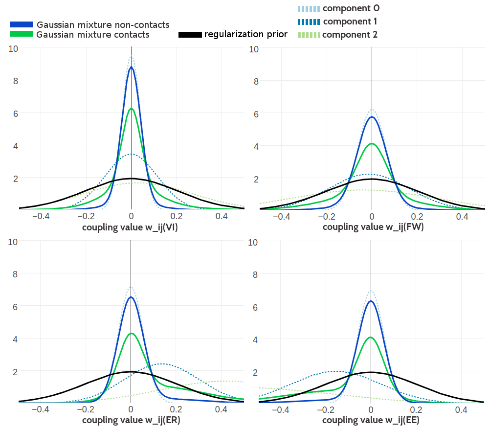
Figure G.6: Visualisation of one-dimensional projections of the three-component Gaussian mixture model for the contact-dependent coupling prior. Hyperparameters, $\gamma_k(\cij)$, $\muk$ and $\Lk$, have been trained on 100,000 residue pairs per contact class and using pseudo-likelihood couplings to estimate the Hessian. Green solid line: Gaussian mixture for contacts. Blue solid line: Gaussian mixture for non-contacts. Black solid line: regularization prior with $\lambda_1 \eq 0.2L$ with L being protein length and assumed $L\eq150$. Light blue dashed line: Gaussian component 0. Dark blue dashed line: Gaussian component 1. Light green dashed line: Gaussian component 2. Top Left One dimensional projection for pair (V,I). Top Right One dimensional projection for pair (F,W). Bottom Left One dimensional projection for pair (E,R). Bottom Right One dimensional projection for pair (E,E).

$Visualisation of one-dimensional projections of the three-component Gaussian mixture model for the contact-dependent coupling prior. Hyperparameters, $\gamma_k(\cij)$, $\muk$ and $\Lk$, have been trained on 500,000 residue pairs per contact class and using pseudo-likelihood couplings to estimate the Hessian. Green solid line: Gaussian mixture for contacts. Blue solid line: Gaussian mixture for non-contacts. Black solid line: regularization prior with $\lambda_1 \eq 0.2L$ with L being protein length and assumed $L\eq150$. Light blue dashed line: Gaussian component 0. Dark blue dashed line: Gaussian component 1. Light Green dashed line: Gaussian component 2. Top Left One dimensional projection for pair (V,I). Top Right One dimensional projection for pair (F,W). Bottom Left One dimensional projection for pair (E,R). Bottom Right One dimensional projection for pair (E,E).$

Figure G.7: Visualisation of one-dimensional projections of the three-component Gaussian mixture model for the contact-dependent coupling prior. Hyperparameters, $\gamma_k(\cij)$, $\muk$ and $\Lk$, have been trained on 500,000 residue pairs per contact class and using pseudo-likelihood couplings to estimate the Hessian. Green solid line: Gaussian mixture for contacts. Blue solid line: Gaussian mixture for non-contacts. Black solid line: regularization prior with $\lambda_1 \eq 0.2L$ with L being protein length and assumed $L\eq150$. Light blue dashed line: Gaussian component 0. Dark blue dashed line: Gaussian component 1. Light Green dashed line: Gaussian component 2. Top Left One dimensional projection for pair (V,I). Top Right One dimensional projection for pair (F,W). Bottom Left One dimensional projection for pair (E,R). Bottom Right One dimensional projection for pair (E,E).

$Visualisation of one-dimensional projections of the three-component Gaussian mixture model for the contact-dependent coupling prior. Hyperparameters, $\gamma_k(\cij)$, $\muk$ and $\Lk$, have been trained on 100,000 residue pairs per contact class and using contrastive divergence couplings to estimate the Hessian. Green solid line: Gaussian mixture for contacts. Blue solid line: Gaussian mixture for non-contacts. Black solid line: regularization prior with $\lambda_1 \eq 0.2L$ with L being protein length and assumed $L\eq150$. Light blue dashed line: Gaussian component 0. Dark blue dashed line: Gaussian component 1. Light green dashed line: Gaussian component 2. Top Left One dimensional projection for pair (V,I). Top Right One dimensional projection for pair (F,W). Bottom Left One dimensional projection for pair (E,R). Bottom Right One dimensional projection for pair (E,E).$

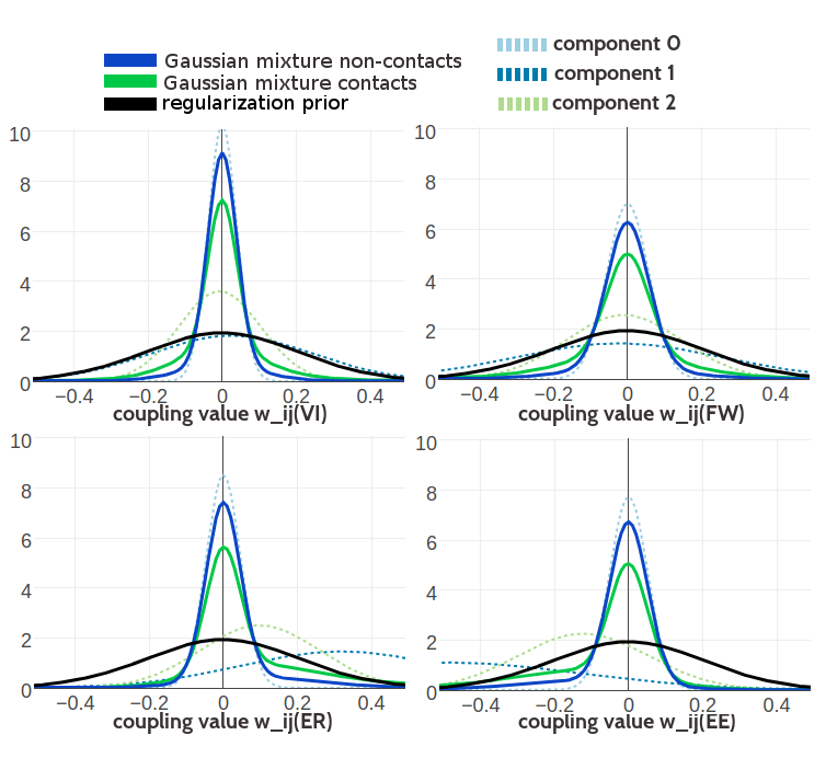
Figure G.8: Visualisation of one-dimensional projections of the three-component Gaussian mixture model for the contact-dependent coupling prior. Hyperparameters, $\gamma_k(\cij)$, $\muk$ and $\Lk$, have been trained on 100,000 residue pairs per contact class and using contrastive divergence couplings to estimate the Hessian. Green solid line: Gaussian mixture for contacts. Blue solid line: Gaussian mixture for non-contacts. Black solid line: regularization prior with $\lambda_1 \eq 0.2L$ with L being protein length and assumed $L\eq150$. Light blue dashed line: Gaussian component 0. Dark blue dashed line: Gaussian component 1. Light green dashed line: Gaussian component 2. Top Left One dimensional projection for pair (V,I). Top Right One dimensional projection for pair (F,W). Bottom Left One dimensional projection for pair (E,R). Bottom Right One dimensional projection for pair (E,E).

$Visualisation of two-dimensional projections of the three-component Gaussian mixture model for the contact-dependent coupling prior.Hyperparameters, $\gamma_k(\cij)$, $\muk$ and $\Lk$, have been trained on 300,000 residue pairs per contact class and using contrastive divergence couplings to estimate the Hessian. 10,000 paired couplings have been sampled from the Gaussian mixture model. The different colors represent the generating component and color code is specified in the legend. Top Left Two-dimensional projection for pairs (E,R) and (R-E) for contacts (using component weight $g_k(1)$). Top Right Two- dimensional projection for pairs (E,E) and (R,E) for contacts (using component weight $g_k(1)$). Bottom Left Two-dimensional projection for pairs (I,L) and (V,I) for contacts (using component weight $g_k(1)$). Bottom Right Two-dimensional projection for pair (I,L) and (V,I) for non-contacts (using component weight $g_k(0)$).$

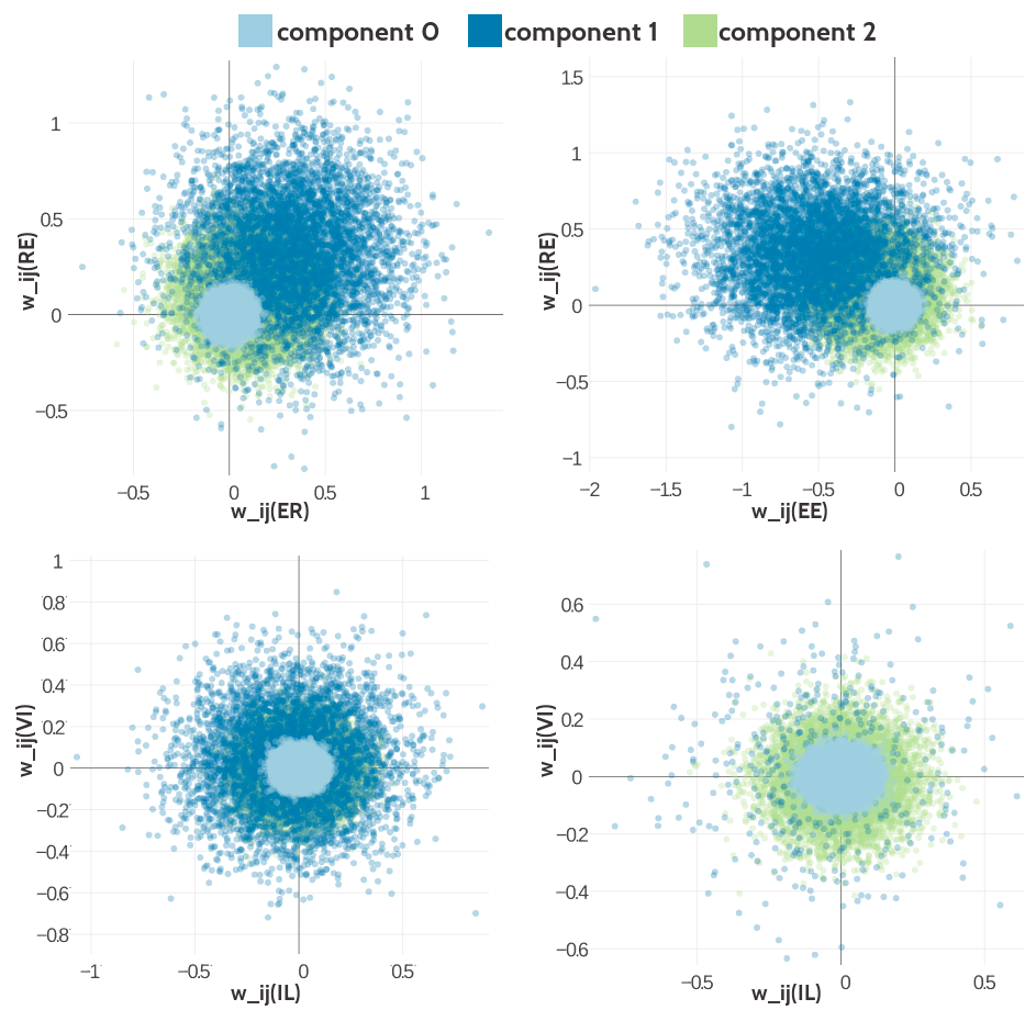
Figure G.9: Visualisation of two-dimensional projections of the three-component Gaussian mixture model for the contact-dependent coupling prior.Hyperparameters, $\gamma_k(\cij)$, $\muk$ and $\Lk$, have been trained on 300,000 residue pairs per contact class and using contrastive divergence couplings to estimate the Hessian. 10,000 paired couplings have been sampled from the Gaussian mixture model. The different colors represent the generating component and color code is specified in the legend. Top Left Two-dimensional projection for pairs (E,R) and (R-E) for contacts (using component weight $g_k(1)$). Top Right Two- dimensional projection for pairs (E,E) and (R,E) for contacts (using component weight $g_k(1)$). Bottom Left Two-dimensional projection for pairs (I,L) and (V,I) for contacts (using component weight $g_k(1)$). Bottom Right Two-dimensional projection for pair (I,L) and (V,I) for non-contacts (using component weight $g_k(0)$).

$Statistics for the hyperparameters, $\gamma_k(\cij)$, $\muk$ and $\Lk$ obtained after 2605 iterations. Trained on 100,000 residue pairs per contact class for a five component Gaussian mixture and using contrastive divergence couplings to estimate the Hessian. Left Component weights $\gamma_k(\cij)$ for residue pairs not in physical contact ($\cij \eq 0$) and true contacts ($\cij \eq 1$). Center Distribution of the 400 elements in the mean vectors $\muk$. Right Distribution of the 400 standard deviations corresponding to the square root of the diagonal of $\Lk^{-1}$.$

Figure G.10: Statistics for the hyperparameters, $\gamma_k(\cij)$, $\muk$ and $\Lk$ obtained after 2605 iterations. Trained on 100,000 residue pairs per contact class for a five component Gaussian mixture and using contrastive divergence couplings to estimate the Hessian. Left Component weights $\gamma_k(\cij)$ for residue pairs not in physical contact ($\cij \eq 0$) and true contacts ($\cij \eq 1$). Center Distribution of the 400 elements in the mean vectors $\muk$. Right Distribution of the 400 standard deviations corresponding to the square root of the diagonal of $\Lk^{-1}$.

$Statistics for the hyperparameters, $\gamma_k(\cij)$, $\muk$ and $\Lk$ obtained after 1229 iterations. Trained on 300,000 residue pairs per contact class for a five component Gaussian mixture and using contrastive divergence couplings to estimate the Hessian. Left Component weights $\gamma_k(\cij)$ for residue pairs not in physical contact ($\cij \eq 0$) and true contacts ($\cij \eq 1$). Center Distribution of the 400 elements in the mean vectors $\muk$. Right Distribution of the 400 standard deviations corresponding to the square root of the diagonal of $\Lk^{-1}$.$

Figure G.11: Statistics for the hyperparameters, $\gamma_k(\cij)$, $\muk$ and $\Lk$ obtained after 1229 iterations. Trained on 300,000 residue pairs per contact class for a five component Gaussian mixture and using contrastive divergence couplings to estimate the Hessian. Left Component weights $\gamma_k(\cij)$ for residue pairs not in physical contact ($\cij \eq 0$) and true contacts ($\cij \eq 1$). Center Distribution of the 400 elements in the mean vectors $\muk$. Right Distribution of the 400 standard deviations corresponding to the square root of the diagonal of $\Lk^{-1}$.

$Visualisation of one-dimensional projections of the five-component Gaussian mixture model for the contact-dependent coupling prior. Hyperparameters, $\gamma_k(\cij)$, $\muk$ and $\Lk$, have been trained on 300,000 residue pairs per contact class and using contrastive divergence couplings to estimate the Hessian. Green solid line: Gaussian mixture for contacts. Blue solid line: Gaussian mixture for non-contacts. Black solid line: regularization prior with $\lambda_1 \eq 0.2L$ with L being protein length and assumed $L\eq150$. Light blue dashed line: Gaussian component 0. Dark blue dashed line: Gaussian component 1. Light green dashed line: Gaussian component 2. Dark green dashed line: Gaussian component 3. Light pink dashed line: Gaussian component 4. Top Left One dimensional projection for pair (V,I). Top Right One dimensional projection for pair (F,W). Bottom Left One dimensional projection for pair (E,R). Bottom Right One dimensional projection for pair (E,E).$

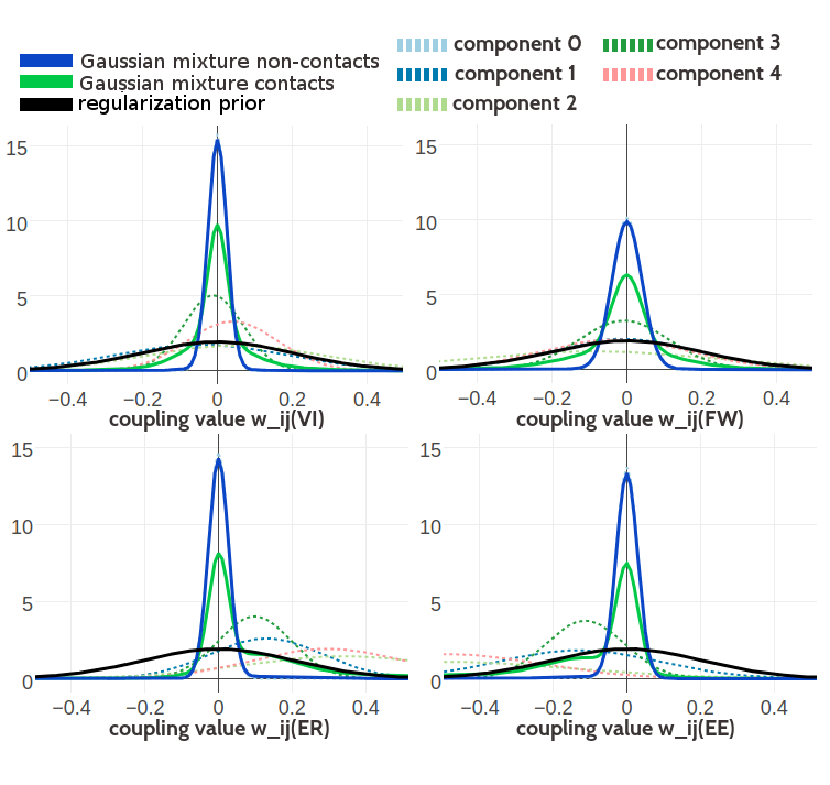
Figure G.12: Visualisation of one-dimensional projections of the five-component Gaussian mixture model for the contact-dependent coupling prior. Hyperparameters, $\gamma_k(\cij)$, $\muk$ and $\Lk$, have been trained on 300,000 residue pairs per contact class and using contrastive divergence couplings to estimate the Hessian. Green solid line: Gaussian mixture for contacts. Blue solid line: Gaussian mixture for non-contacts. Black solid line: regularization prior with $\lambda_1 \eq 0.2L$ with L being protein length and assumed $L\eq150$. Light blue dashed line: Gaussian component 0. Dark blue dashed line: Gaussian component 1. Light green dashed line: Gaussian component 2. Dark green dashed line: Gaussian component 3. Light pink dashed line: Gaussian component 4. Top Left One dimensional projection for pair (V,I). Top Right One dimensional projection for pair (F,W). Bottom Left One dimensional projection for pair (E,R). Bottom Right One dimensional projection for pair (E,E).

$Visualisation of two-dimensional projections of the five-component Gaussian mixture model for the contact-dependent coupling prior. Hyperparameters, $\gamma_k(\cij)$, $\muk$ and $\Lk$, have been trained on 300,000 residue pairs per contact class and using contrastive divergence couplings to estimate the Hessian. 10,000 values have been samples from the Gaussian mixture model. Light blue: values that have been generated by zero component. Dark blue: values that have been generated by Gaussian component 1. Light green: values that have been generated by Gaussian component 3. Dark green: values that have been generated by Gaussian component 4. Light pink: values that have been generated by Gaussian component 4. Top Left Two-dimensional projection for pairs (E,R) and (R-E) for contacts (using component weight $g_k(1)$). Top Right Two- dimensional projection for pairs (E,E) and (R,E) for contacts (using component weight $g_k(1)$). Bottom Left Two-dimensional projection for pairs (I,L) and (V,I) for contacts (using component weight $g_k(1)$). Bottom Right Two-dimensional projection for pair (I,L) and (V,I) for non-contacts (using component weight $g_k(0)$).$

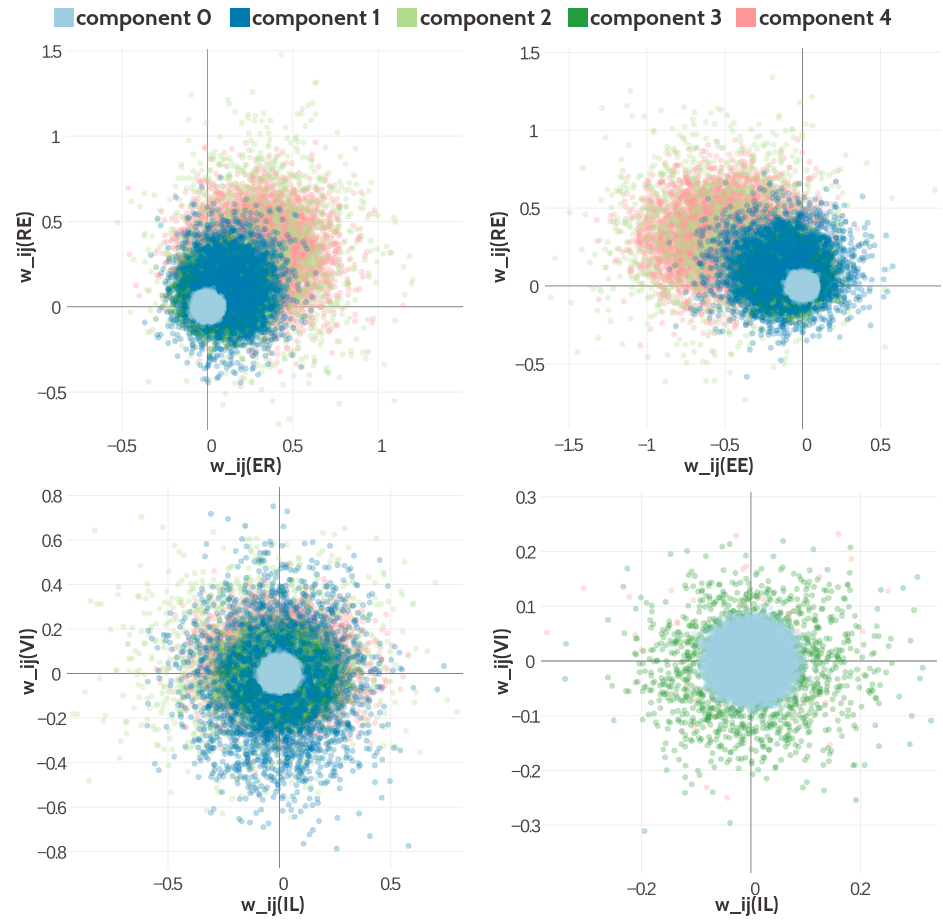
Figure G.13: Visualisation of two-dimensional projections of the five-component Gaussian mixture model for the contact-dependent coupling prior. Hyperparameters, $\gamma_k(\cij)$, $\muk$ and $\Lk$, have been trained on 300,000 residue pairs per contact class and using contrastive divergence couplings to estimate the Hessian. 10,000 values have been samples from the Gaussian mixture model. Light blue: values that have been generated by zero component. Dark blue: values that have been generated by Gaussian component 1. Light green: values that have been generated by Gaussian component 3. Dark green: values that have been generated by Gaussian component 4. Light pink: values that have been generated by Gaussian component 4. Top Left Two-dimensional projection for pairs (E,R) and (R-E) for contacts (using component weight $g_k(1)$). Top Right Two- dimensional projection for pairs (E,E) and (R,E) for contacts (using component weight $g_k(1)$). Bottom Left Two-dimensional projection for pairs (I,L) and (V,I) for contacts (using component weight $g_k(1)$). Bottom Right Two-dimensional projection for pair (I,L) and (V,I) for non-contacts (using component weight $g_k(0)$).

Figure G.14: Mean precision for top ranked contact predictions over 500 proteins. The “Bayesian Posterior” methods compute the posterior probability of contacts with the Bayesian framework employing a three component Gaussian mixture coupling prior based on couplings computed with pseudo-likelihood. Hyperparameters for the coupling prior have been trained on different dataset sizes as specified in the legend. Furthermore residue pairs not in physical contact are defined either by $25 \angstrom$ or a $8 \angstrom \Cb$ distance cutoff that is also specified in the legend. Bayesian Posterior 100k, non-contacts 5 : Bayesian model trained on 100,000 contacts and 500,000 non-contacts with non-contacts defined by an $25 \angstrom \Cb$ distance threshold.

Figure G.15: Mean precision for top ranked contact predictions over 500 proteins. The “Bayesian Posterior” methods compute the posterior probability of contacts with the Bayesian framework employing a three component Gaussian mixture coupling prior based on couplings computed with contrastive divergence. Hyperparameters for the coupling prior have been trained on different dataset sizes as specified in the legend. random forest (pLL) random forest model trained on sequence features and and additional pseudo-likelihood contact score feature. Bayesian Posterior 100k: Bayesian model trained on 100,000 residue pairs per contact class. Bayesian Posterior 300k: Bayesian model trained on 300,000 residue pairs per contact class. Bayesian Posterior 500k: Bayesian model trained on 500,000 residue pairs per contact class. pseudo-likelihood: contact score is computed as APC corrected Frobenius norm of the couplings computed from pseudo-likelihood.

Figure G.16: Mean precision for top ranked contact predictions over 500 proteins. The “Bayesian Posterior” methods compute the posterior probability of contacts with the Bayesian framework employing a Gaussian mixture coupling prior based on couplings computed with contrastive divergence. Hyperparameters for the coupling prior have been trained on 100,000 residue pairs per contact class. The number of Gaussian components in the Gaussian mixture model is specified in the legend. random forest (pLL) random forest model trained on sequence features and and additional pseudo-likelihood contact score feature. Bayesian Posterior 3: Bayesian model utilizing a three component Gaussian mixture. Bayesian Posterior 5: Bayesian model utilizing a five component Gaussian mixture. Bayesian Posterior 10: Bayesian model utilizing a ten component Gaussian mixture. pseudo-likelihood: contact score is computed as APC corrected Frobenius norm of the couplings computed from pseudo-likelihood.

Figure G.17: Mean precision for top ranked contact predictions over 500 proteins splitted into four equally sized subsets with respect to Neff. Upper left: Subset of proteins with Neff < Q1. Upper right: Subset of proteins with Q1 <= Neff < Q2. Lower left: Subset of proteins with Q2 <= Neff < Q3. Lower right: Subset of proteins with Q3 <= Neff < Q4. random forest (pLL) random forest model trained on sequence features and and additional pseudo-likelihood contact score feature. Bayesian Posterior pLL: Bayesian model computing the posterior probability of contacts with a three component Gaussian mixture coupling prior based on pseudo-likelihood couplings. Hyperparameters for the coupling prior have been trained on 300,000 residue pairs per contact class. Bayesian Posterior CD: Bayesian model computing the posterior probability of contacts with a three component Gaussian mixture coupling prior based on contrastive divergence couplings. Hyperparameters for the coupling prior have been trained on 300,000 residue pairs per contact class. pseudo-likelihood: contact score is computed as APC corrected Frobenius norm of the couplings computed from pseudo-likelihood.

Figure G.18: Precision of top ranked contact predictions for protein 1c75A00. pseudo-likelihood: Contact scores are computed as the APC corrected Frobenius norm of the pseudo-likelihood couplings. contrastive divergence: Posterior probabilities computed with a three component Gaussian mixture coupling prior based on pseudo-likelihood couplings.

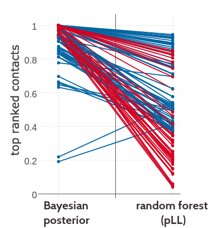
Comparing the ranking of highest scoring contacts predicted with Bayesian model using the posterior probability estimates for contacts and the random forest model trained on sequence features and pseudo-likelihood contact scores computed as APC corrected Frobenius norm of the couplings. Plot shows predictions for the top 71 (=L) predictions from either method. Identical residue pairs are connected with a line. Green indicates identical ranking of the residue pair for both methods. Blue indicates higher ranking of the residue pair for random forest model. Red indicates higher ranking of the residue pair for Bayesian model.

Figure G.19: Comparing the ranking of highest scoring contacts predicted with Bayesian model using the posterior probability estimates for contacts and the random forest model trained on sequence features and pseudo-likelihood contact scores computed as APC corrected Frobenius norm of the couplings. Plot shows predictions for the top 71 (=L) predictions from either method. Identical residue pairs are connected with a line. Green indicates identical ranking of the residue pair for both methods. Blue indicates higher ranking of the residue pair for random forest model. Red indicates higher ranking of the residue pair for Bayesian model.

Figure G.20: Probabilities for protein 1c75A00 predicted with Bayesian model using the posterior probability estimates for contacts and the random forest model trained on sequence features and pseudo-likelihood contact scores computed as APC corrected Frobenius norm of the couplings.