3.1 Approximating the Gradient of the Full Likelihood with Contrastive Divergence

The gradient of the regularized full log likelihood with respect to the couplings \(\wijab\) can be written as \[\begin{equation} \frac{\partial \LLreg}{\partial \wijab} = \; N_{ij} q(x_i \eq a, x_j=b) - N_{ij} \; p(x_i \eq a, x_j \eq b | \v,\w) - \lambda_w \wijab \; , \tag{3.1} \end{equation}\]

where \(N_{ij} q(x_i \eq a, x_j=b)\) are the empirical pairwise amino acid counts, \(p(x_i \eq a, x_j \eq b | \v,\w)\) corresponds to the marginal distribution of the Potts model and \(\lambda_w \wijab\) is the partial derivative of the L2-regularizer used to constrain the couplings \(\w\). The empirical amino acid counts are constant and need to be computed only once from the alignment. The model probability term cannot be computed analytically as it involves the partition function that has exponential complexity.

MCMC algorithms are predominantly used in Bayesian statistics to generate samples from probability distributions that involve the computation of complex integrals and therefore cannot be computed analytically [94,193]. Samples are generated from a probability distribution as the current state of a running Markov chain. If the Markov chain is run long enough, the equilibrium statistics of the samples will be identical to the true probability distribution statistics. In 2002, Lapedes et al. applied MCMC sampling to approximate the probability terms in the gradient of the full likelihood [103]. They obtained sequence samples from a Markov chain that was run for 4,000,000 steps by keeping every tenth configuration of the chain. Optimization converged after 10,000 - 15,000 epochs when the gradient had become zero. The expected amino acid counts according to the model distribution, \(N_{ij} \; p(x_i \eq a, x_j \eq b | \v,\w)\), were estimated from the generated samples. Their approach was successfull but is computationally feasible only for small proteins and points out the limits of applying MCMC algorithms. Typically, they require many sampling steps to obtain unbiased estimates from the stationary distribution which comes at high computational costs.

In 2002, Hinton invented Contrastive Divergence as an approximation to MCMC methods [192]. It was originally developed for training products of experts models but it can generally be applied to maximizing log likelihoods and has become popular for training restricted Boltzmann machines [94,194,195]. The idea is simple: instead of starting a Markov chain from a random point and running it until it has reached the stationary distribution, it is initialized with a data sample and evolved for only a small number of steps. Obviously the chain has not yet converged to its stationary distribution and the data sample obtained from the current configuration of the chain presents a biased estimate. The intuition behind CD is, that eventhough the gradient estimate is noisy and biased, it points roughly into a similar direction as the true gradient of the full likelihood. Therefore the approximate CD gradient should become zero approximately where the true gradient of the likelihood becomes zero. Once the parameters are close to the optimum, starting a Gibbs chain from a data sample should reproduce the empirical distribution and not lead away from it, because the parameters already describe the empirical distribution correctly.

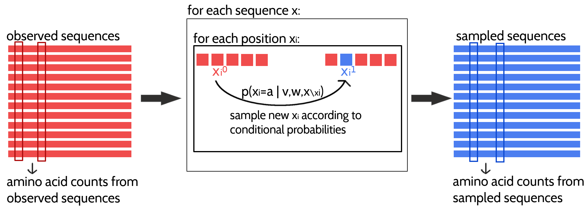
The approximation of the likelihood gradient with CD according to the Potts model for modelling protein families is visualized in Figure 3.1. \(N\) Markov chains will be initialized with the \(N\) sequences from the MSA and \(N\) new samples will be generated by a single step of Gibbs sampling from each of the \(N\) sequences. One full step of Gibbs sampling updates every sequence position \(i \in \{1, \ldots, L\}\) subsequently by randomly selecting an amino acid based on the conditional probabilities for observing an amino acid \(a\) at position \(i\) given the model parameters and all other (already updated) sequence positions: \[\begin{equation} p(\seq_i = a | (x_1, \ldots, x_{i-1}, x_{i+1}, \ldots, x_L), \v, \w) \propto \exp \left( \vi(a) + \sum_{\substack{j=1 \\ i \ne j}}^L \wij(a, x_j) \right) \tag{3.2} \end{equation}\]

The generated sample sequences are then used to compute the pairwise amino acid frequencies that correspond to rough estimates of the marginal probabilities of the Potts model. Finally, an approximate gradient of the full likelihood is obtained by subtracting the sampled amino acid counts from the empirical amino acid counts as denoted in eq. (3.1).

Figure 3.1: Approximating the full likelihood gradient of the Potts model with CD. Pairwise amino acid counts are computed from the observed sequences of the input alignment shown in red on the left. Expected amino acid frequencies according to the model distribution are computed from a sampled alignment shown in blue on the right. The CD approximation of the likelihood gradient is obtained by computing the difference in amino acid counts of the observed and sampled alignment. A newly sampled sequence is obtained by evolving a Markov chain, that is initialized with an observed sequence, for one full Gibbs step. The Gibbs step involves updating every position in the sequence (unless it is a gap) according to the conditional probabilities for the 20 amino acids at this position.

The next sections elucidate the optimization of the Potts model full likelihood with CD to obtain an approximation to the gradient.

References

94. Murphy, K.P. (2012). Machine Learning: A Probabilistic Perspective (MIT Press).

193. Andrieu, C., Freitas, N. de, Doucet, A., and Jordan, M.I. (2003). An Introduction to MCMC for Machine Learning. Mach. Learn. 50, 5–43., doi: 10.1023/A:1020281327116.

103. Lapedes, A., Giraud, B., and Jarzynski, C. (2012). Using Sequence Alignments to Predict Protein Structure and Stability With High Accuracy.

192. Hinton, G.E. (2002). Training Products of Experts by Minimizing Contrastive Divergence. Neural Comput. 14, 1771–1800., doi: doi:10.1162/ 089976602760128018.

194. Fischer, A., and Igel, C. (2012). An Introduction to Restricted Boltzmann Machines. Lect. Notes Comput. Sci. Prog. Pattern Recognition, Image Anal. Comput. Vision, Appl. 7441, 14–36., doi: 10.1007/978-3-642-33275-3_2.

195. Bengio, Y., and Delalleau, O. (2009). Justifying and Generalizing Contrastive Divergence. Neural Comput. 21, 1601–21., doi: 10.1162/neco.2008.11-07-647.