3.4 Using ADAM to Optimize Contrastive Divergence

ADAM computes per-parameter adaptive learning rates including momentum. The default values have been found to work well in practice so that little parameter tuning is required (see methods section 3.7.5.1 for details) [196,211]. However, I tested ADAM with different learning rates for the optimization with CD-1 for protein 1mkcA00 (number of sequences = 142) and 1c75A00 (number of sequences = 28078) and found that both proteins are sensitive to the choice of learning rate. In contrast to plain stochastic gradient descent, with ADAM it is possible to use larger learning rates for proteins having large alignments, because the learning rate will be adapted to the magnitude of the gradient for every parameter individually. For protein 1mkcA00, with Neff=96, a learning rate of 5e-3 quickly leads to convergence whereas for protein 1c75A00, having Neff=16808, an even larger learning rate can be chosen to obtain quick convergence (see Appendix Figure E.16). Therefore, I again specified the learning rate as a function of Neff, \(\alpha = 2\mathrm{e}{-3}\log(\text{N}_{\text{eff}})\), such that for small Neff, e.g. 5th percentile of the distribution in the dataset \(\approx 50\), this definition of the learning rate yields \(\alpha_0 \approx 8\mathrm{e}{-3}\) and for large Neff, e.g. 95th percentile \(\approx 15000\), this yields \(\alpha_0 \approx 2\mathrm{e}{-2}\).

It is interesting to note, that the norm of the coupling parameters, \(||\w||_2\), converges towards different values depending on the choice of the learning rate (see Appendix Figure E.16. By default, ADAM uses a constant learning rate, because the algorithm performs a kind of step size annealing by nature. However, popular implementations of ADAM in the Keras [212] and Lasagne [213] packages allow the use of an annealing schedule. I therefore tested ADAM with a sigmoidal learning rate annealing schedule which already gave good results for SGD (see section 3.2.2). Indeed, as can be seen in Appendix Figure E.17, when ADAM is used with a sigmoidal decay of the learning rate, the L2-norm of the coupling parameters \(||\w||_2\) converges roughly towards the same value. For the following analysis I used ADAM with a learning rate defined as a function of Neff and a sigmoidal learning rate annealing schedule with decay rate \(\gamma \eq 5e-6\).

I evaluated CD-1, CD-10 and persistent contrastive divergence. As before, I will also evaluate a combination of both, such that PCD is switched on, when the relative change of the norm of coupling parameters, \(||\w||_2\), falls below a small threshold. Figure 3.18 shows the benchmark for training the various modified CD models with the ADAM optimizer. Overall, the predictive performance for CD and PCD did not improve by using the ADAM optimzier instead of the manually tuned stochastic gradient descent optimizer. Therefore it can be concluded that adaptive learning rates and momentum do not provide an essential advantage for inferring Potts model parameters with CD and PCD.

Figure 3.18: Mean precision for top ranked contact predictions over 300 proteins. Contact score is computed as APC corrected Frobenius norm of the couplings. pseudo-likelihood: couplings computed from pseudo-likelihood. CD ADAM: couplings computed from contrastive divergence using ADAM optimizer. CD ADAM #Gibbs steps = 10: couplings computed from contrastive divergence using ADAM optimizer and 10 Gibbs steps for sampling sequences. pCD ADAM: couplings computed from persistent contrastive divergence usign ADAM optimizer. pCD ADAM start = 1e-3: ADAM starts by optimizing the full likelihood using the CD gradient estimate and switches to the PCD gradient estimate once the relative change of L2 norm of parameters has fallen below \(\epsilon \eq \mathrm{1e}{-3}\) evaluated over the last 10 iterations. pCD ADAM start = 1e-5: same as “pCD ADAM start = 1e-3” but PCD is switched on for \(\epsilon \eq \mathrm{1e}{-5}\)

The convergence analysis for the two example proteins 1ahoA00 and 1c75A00 reveals, that optimization with ADAM converges towards similar offsets as optimization with plain SGD with respect to the L2 norm of coupling parameters. For 1ahoA00, with low Neff=229, the L2 norm of the parameters converges towards \(||\w||_2 \approx 21.6\) when using CD-1 and towards \(||\w||_2 \approx 24\) when using PCD or CD-k with k>1 (compare left plots in Figures 3.19 and 3.17). For protein 1c75A00, with high Neff=16808, ADAM seems to find distinct optima that are clearly separated in contrast to using plain SGD. When using ADAM with CD-1 the algorithm converges towards \(||\w||_2 \approx 120\), ADAM with CD-5 converges towards \(||\w||_2 \approx 130\) and with CD-10 towards \(||\w||_2 \approx 131\). And using ADAM with PCD, regardless of whether the PCD gradient estimate is used right from the start of optimization or only later, the algorithm converges towards \(||\w||_2 \approx 134\). Therefore, ADAM establishes the clear trend that longer sampling, or sampling with persistent chaisn results in larger parameter estimates.

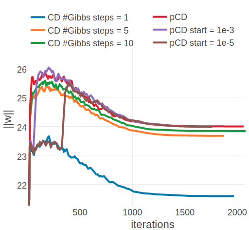
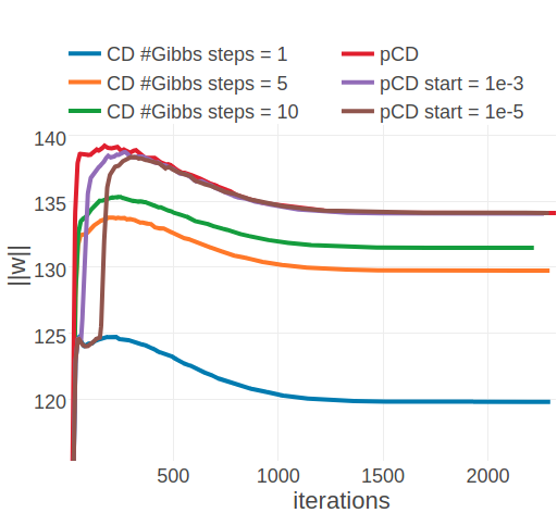
Figure 3.19: Monitoring the L2 norm of coupling parameters,\(||\w||_2\), for protein 1ahoA00 and 1c75A00 during optimization of CD and PCD with the ADAM optimizer. Contrastive Divergence (CD in legend) is optimized employing a different number of Gibbs steps that are specified in the legend. Persistent contrastive divergence (pCD in legend) uses one Gibbs step. “pCD start= X” indicates that optimization starts by using the CD gradient estimate and switches to the PCD gradient estimate once the relative change of L2 norm of parameters has fallen below a small threshold over the last 10 iterations. The threshold is given in the legend. Left Protein 1ahoA00 has length L=64 and 378 sequences in the alignment (Neff=229) Right Protein 1c75A00 has length L=71 and 28078 sequences in the alignment (Neff=16808).

3.4.1 A Potts model specific convergence criterion

For the Potts model there exists a necessary but not sufficient condition that is satisfied at the optimum when the gradient is zero (derived in method section 3.7.4) and that is given by, \(\sum_{a,b=1}^{20} \wijab = 0\). This condition is never violated, as long as parameters satisfy this criterion at initialization and the same step size is used to update all parameters. To understand why, note that the 400 partial derivatives \(\frac{\partial L\!L(\v^*, \w)}{\partial \wijab}\) for a residue pair \((i,j)\) and for \(a,b \in \{1, \ldots, 20\}\) are not independent. The sum over the 400 pairwise amino acid counts at positions \(i\) and \(j\) is identical for the observed and the sampled alignment and amounts to, \(\sum_{a,b=1}^{20} N_{ij} q(x_i \eq a, q_j \eq b) = N_{ij}\).

Considering a residue pair \((i,j)\) and assuming amino acid pair \((a,b)\) has higher counts in the sampled alignment than in the observed input alignment, then this difference in counts must be compensated by other amino acid pairs \((c,d)\) having less counts in the sampled alignment compared to the true alignment (see Figure 3.20). Therefore, it holds \(\sum_{a,b=1}^{20} \frac{\partial L\!L(\v^*, \w)}{\partial \wijab} = 0\). This symmetry is translated into parameter updates as long as the same step size is used to update all parameters. However, when using adaptive learning rates, e.g. with the ADAM optimizer, this symmetry is broken and the condition \(\sum_{a,b=1}^{20} \wijab = 0\) can be violated during the optimization processs.

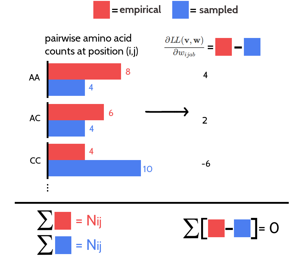
Figure 3.20: The 400 partial derivatives \(\frac{\partial \LLreg(\v^*,\w)}{\partial \wijab}\) at position \((i,j)\) for \(a,b \in \{1, \ldots, 20 \}\) are not independent. Red bars represent pairwise amino acid counts at position \((i,j)\) for the empirical alignment. Blue bars represent pairwise amino acid counts at position \((i,j)\) for the sampled alignment. The sum over pairwise amino acid counts at position \((i,j)\) for both alignments is \(N_{ij}\), which is the number of ungapped sequences. The partial derivative for \(\wijab\) is computed as the difference of pairwise amino acid counts for amino acids \(a\) and \(b\) at position \((i,j)\). The sum over the partial derivatives \(\frac{\partial \LLreg(\v^*,\w)}{\partial \wijab}\) at position \((i,j)\) for all \(a,b \in \{1, \ldots, 20 \}\) is zero.

For proteins 1ahoA00 and 1c75A00, Figure 3.21 shows the number of residue pairs for which this condition is violated according to \(|\sum_{a,b=1}^{20} \wijab| > \mathrm{1e}{-2}\), during optimization with ADAM. For about half out of the 2016 residue pairs in protein 1ahoA00 the condition is violated at the end of optimization. For protein 1c75A00 it is about 2300 out of the 2485 residue pairs. Whereas this is not a problem when computing the contact score based on the Frobenius norm of the coupling matrix, it is problematic when utilizing the couplings in the Bayesian framework presented in section 5, which requires the condition \(\sum_{a,b=1}^{20} \wijab = 0\) to hold.

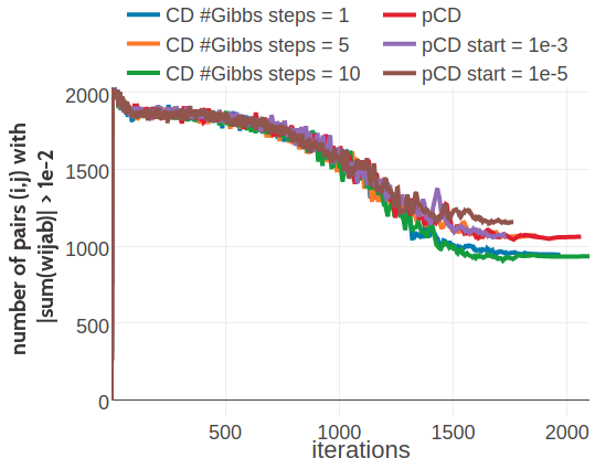
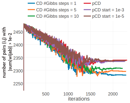
Figure 3.21: Monitoring the number of residue pairs for which \(|\sum_{a,b=1}^{20} \wijab| > \mathrm{1e}{-2}\). Legend is the same as in Figure 3.19. Left Protein 1ahoA00 has length L=64 and 378 sequences in the alignment (Neff=229) Right Protein 1c75A00 has length L=71 and 28078 sequences in the alignment (Neff=16808).

References

196. Ruder, S. (2017). An overview of gradient descent optimization algorithms. arXiv.

211. Kingma, D., and Ba, J. (2014). Adam: A Method for Stochastic Optimization.

212. Chollet, F. others (2015). Keras.

213. Dieleman, S., Schlüter, J., Raffel, C., Olson, E., Sønderby, S.K., Nouri, D., Maturana, D., Thoma, M., Battenberg, E., and Kelly, J. et al. (2015). Lasagne: First release., doi: 10.5281/ZENODO.27878.