PhD thesis: residue-residue contact prediction

1.4 Evaluating Contact Prediction Methods

Choosing an appropriate benchmark for contact prediction is determined by the further utilization of the predictions. Most prominently, predicted contacts are used to assist structure prediction as outlined in the last section 1.3. Therefore, one could assess the quality of structural models computed with the help of predicted contacts. However, predicting structural models adds not only another layer of computational complexity but also raises questions about implementation details of the folding protocol.

It has been found that in general a small number of accurate contacts is sufficient to constrain the overal protein fold as already discussed. From these considerations emerged various standard benchmarks that have been established by the CASP community over many years [90,172,173]. CASP, the well-respected and independent competition for the structural bioinformatic’s community introduced the contact prediction category in 1996. Taking place every two years, the progress in the field is assessed in a blind competition and the community discusses the outcome in a subsequent meeting. According to the CASP regulations, a pair of residues is defined to be in physical contact when the distance between their $\Cb$ atoms ($C_{\alpha}$ in case of glycine) is less than $8 \angstrom$ in the reference protein structure.

The overall performance of a contact predictor is evaluated by the mean precision over a testset of proteins with known high quality 3D structures against the top scoring predictions from every protein. The number of top scoring predictions per protein is typically normalized with respect to protein length $L$ and precision is defined as the number of true contacts among the top scoring predicted contacts,

\[\begin{equation} \textrm{precision} = \frac{TP}{TP + FP} \; , \end{equation}\]

where $TP$ is a true positive contact and $FP$ is false positive contact. A popular variant of this benchmark plot shows the mean precision of a certain fraction of top ranked predictions (e.g. L/5 top ranked predictions) against specific properties of the test proteins such as protein length or alignment depth [174]. Another informative metric is mean error defined as:

\[\begin{equation} \textrm{mean error} = \frac{\textrm{error}}{TP + FP} \begin{cases} error = \Delta\Cb - T & \text{if } \Delta\Cb > T\\ error = 0, &\text{otherwise } \end{cases} \end{equation}\]

where $\Delta\Cb$ is the actual distance of a residue pair in the native structure, and $T$ is the distance threshold defining a true contact. The mean error helps to asses how wrong false positive predictions are. During CASP11 further evaluation metrics have been introduced, such as Matthews correlation coefficient, area under the precision-recall curve or F1 measure but they are rarely used in studies [90].

Currently best methods perform in the range XXX. Sequence feature based methods: Their performance is less dependent on the number of available sequence homologs compared to coevolution methods and therefore they can outperform pure coevolution methods in low data ranges [71,175]. TODOOOPLOT

1.4.1 Sequence Separation

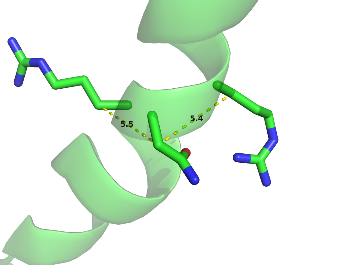
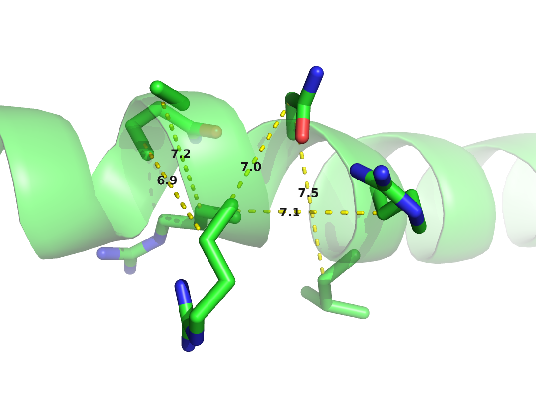
Local residue pairs separated by only some positions in sequence (e.g $|i-j| < 6$) are usually filtered out for evaluating contact prediction methods. They are trivial to predict as they typically correspond to contacts within secondary structure elements and reflect the local geometrical constraints. Figure 1.8 shows the distribution of $\Cb$ distances for various minimal sequence separation thresholds. Without filtering local residue pairs (sequence separation 1), there are several additional peaks in the distribution around $5.5\angstrom$, $7.4\angstrom$ and $10.6\angstrom$ that can be attributed to local interactions in e.g. helices (see Figure 1.9).

Figure 1.8: Distribution of residue pair $\Cb$ distances over 6741 proteins in the dataset (see Methods 2.6.1) at different minimal sequence separation thresholds.

$$\Cb$ distances between neighboring residues in $\alpha$-helices. Left: Direct neighbors in $\alpha$-helices have $\Cb$ distances around $5.4\angstrom$ due to the geometrical constraints from $\alpha$-helical architecture. Right: Residues separated by two positions ($|i-j| = 2$) are less geometrically restricted to $\Cb$ distances between $7\angstrom$ and $7.5\angstrom$.$ $$\Cb$ distances between neighboring residues in $\alpha$-helices. Left: Direct neighbors in $\alpha$-helices have $\Cb$ distances around $5.4\angstrom$ due to the geometrical constraints from $\alpha$-helical architecture. Right: Residues separated by two positions ($|i-j| = 2$) are less geometrically restricted to $\Cb$ distances between $7\angstrom$ and $7.5\angstrom$.$

Figure 1.9: $\Cb$ distances between neighboring residues in $\alpha$-helices. Left: Direct neighbors in $\alpha$-helices have $\Cb$ distances around $5.4\angstrom$ due to the geometrical constraints from $\alpha$-helical architecture. Right: Residues separated by two positions ($|i-j| = 2$) are less geometrically restricted to $\Cb$ distances between $7\angstrom$ and $7.5\angstrom$.

Commonly, sequence separation bins are applied to distuinguish short ($6 < |i-j| \le 12$), medium ($12 < |i-j| \le 24$) and long range ($|i-j| > 24$) contacts [90,173]. Especially long range contacts are of importance for structure prediction as they are the most informative and able to constrain the overal fold of a protein [172].

1.4.2 Interpretation of Evaluation Results

There are certain subtleties to be considered when interpreting contact prediction evaluation results.

The rigid $\Cb$ distance definition of a contact is a very rough measure of true physical interactions between amino acid sidechains. More importantly, interactions between sidechains depend on their physico-chemical properties, on their orientation and different environments within proteins (see section ??) [176]. A simple $\Cb$ distance threshold not only misses to reflect biological interaction preferences of amino acids but also provides a questionable gold-standard for benchmarking. Other distance thresholds and definitions for physical contacts (e.g minimal atomic distances or distance between functional groups) have been studied as well. In fact, Duarte and colleagues found that using a $\Cb$ distance threshold between 9$\angstrom$ and 11$\angstrom$ yields optimal results when predicting the 3D structure from the respective contacts [45]. Anishchenko and colleagues analysed false positive predictions with respect to a minimal atom distance threshold $< 5 \angstrom$, as they found that this cutoff optimally defines direct physical interactions of residue pairs [177].

Another issue concerns structural variation within a protein family. Evolutionary couplings are inferred from all family members in the MSA and therefore predicted contacts might be physical contacts in one family member but not in another. Anishchenko et al. could show that more than $80\%$ of false positives at intermediate distances (minimal heavy atom distance 5-15$\angstrom$) are true contacts in at least one homolog structure [177]. Therefore, choosing the right trade-off between sensitivity and specificity when generating alignments is a crucial step as well as choosing the target protein structure for evaluation.

Finally, an important aspect not considered in the standard benchmarks is the spread of predicted contacts. It is perfectly possible to improve precison of predicted contacts without translating this improvement to better structural models. The reason being that structurally redundant contacts, that is contacts in the immediate sequence neighborhood of other contacts, do not give additional information to constrain the fold [39,44,80]. For example, given a contact between residues $i$ and $j$, there is hardly an added value knowing that there is a contact between residues $i\!+\!1$ and $j\!+\!1$ when it comes to predicting the overal topology. This observation is highly relevant for deep learning methods due to their unique ability to abstract higher order interactions and recognize contact patterns. Several measures of the contact spread have been developed, like the mean euclidian distance between true and predicted contacts, but are not commonly evaluated yet [39,144].

References

90. Monastyrskyy, B., D’Andrea, D., Fidelis, K., Tramontano, A., and Kryshtafovych, A. (2015). New encouraging developments in contact prediction: Assessment of the CASP11 results. Proteins., doi: 10.1002/prot.24943.

172. Monastyrskyy, B., Fidelis, K., Tramontano, A., and Kryshtafovych, A. (2011). Evaluation of residue-residue contact predictions in CASP9. Proteins 79 Suppl 1, 119–125., doi: 10.1002/prot.23160.

173. Monastyrskyy, B., D’Andrea, D., Fidelis, K., Tramontano, A., and Kryshtafovych, A. (2014). Evaluation of residue-residue contact prediction in CASP10. Proteins 82 Suppl 2, 138–153.

174. Ashkenazy, H., Unger, R., and Kliger, Y. (2009). Optimal data collection for correlated mutation analysis. Proteins 74, 545–55., doi: 10.1002/prot.22168.

71. Wang, Z., and Xu, J. (2013). Predicting protein contact map using evolutionary and physical constraints by integer programming. Bioinformatics 29, i266–73.

175. Kosciolek, T., and Jones, D.T. (2015). Accurate contact predictions using coevolution techniques and machine learning. Proteins Struct. Funct. Bioinforma., n/a–n/a.

176. Betts, M.J., and Russell, R.B. Amino Acid Properties and Consequences of Substitutions. In Bioinforma. genet. (Chichester, UK: John Wiley & Sons, Ltd), pp. 289–316., doi: 10.1002/0470867302.ch14.

45. Duarte, J.M., Sathyapriya, R., Stehr, H., Filippis, I., and Lappe, M. (2010). Optimal contact definition for reconstruction of contact maps. BMC Bioinformatics 11., doi: 10.1186/1471-2105-11-283.

177. Anishchenko, I., Ovchinnikov, S., Kamisetty, H., and Baker, D. (2017). Origins of coevolution between residues distant in protein 3D structures. Proc. Natl. Acad. Sci., 201702664., doi: 10.1073/pnas.1702664114.

39. Marks, D.S., Colwell, L.J., Sheridan, R., Hopf, T.A., Pagnani, A., Zecchina, R., and Sander, C. (2011). Protein 3D structure computed from evolutionary sequence variation. PLoS One 6, e28766., doi: 10.1371/journal.pone.0028766.

44. Kim, D.E., Dimaio, F., Yu-Ruei Wang, R., Song, Y., and Baker, D. (2014). One contact for every twelve residues allows robust and accurate topology-level protein structure modeling. Proteins 82 Suppl 2, 208–18.

80. Jones, D.T., Singh, T., Kosciolek, T., and Tetchner, S. (2015). MetaPSICOV: combining coevolution methods for accurate prediction of contacts and long range hydrogen bonding in proteins. Bioinformatics 31, 999–1006., doi: 10.1093/bioinformatics/btu791.

144. Oliveira, S.H.P. de, Shi, J., and Deane, C.M. (2016). Comparing co-evolution methods and their application to template-free protein structure prediction. Bioinformatics, btw618., doi: 10.1093/bioinformatics/btw618.